Demo - The Tau method

Mikael Mortensen (email: mikaem@math.uio.no), Department of Mathematics, University of Oslo.

Date: June 15, 2021

Summary. Shenfun has primarily been developed for the spectral Galerkin method. However, there are other methods out there that make use of global basis functions and variational principles. One such method, which has a lot in common with the spectral Galerkin method, is the Tau method. The principle difference between a Tau method and a spectral Galerkin method is in the choice of basis functions. The spectral Galerkin method is usually defined through function spaces where the boundary conditions of the problem are already built in. The tau-method, on the other hand, usually considers only the orthogonal basis, like pure Chebyshev or Legendre polynomials, and derives differentiation matrices for these bases. The boundary conditions are then usually fixed through manipulation of a couple of rows of the differentiation matrix. In this demo we will show how the original tau-method can be easily implemented using shenfun.

The tau method for Poisson’s equation in 1D

Poisson’s equation is given on a domain \(\Omega = (-1, 1)\) as

\[\begin{equation} \nabla^2 u(x) = f(x) \quad \text{for }\, x \in \Omega, \label{eq:poisson} \tag{1} \end{equation}\]

\[\begin{equation} u(-1)=a, u(1)=b, \notag \label{_auto1} \tag{2} \end{equation}\]

where \(u(x)\) is the solution, \(f(x)\) is a function and \(a, b\) are two possibly non-zero constants. To solve Eq. (1) with the tau method we choose either Legendre of Chebyshev basis functions \(\phi_k\), and then look for solutions

\[\begin{equation} u(x) = \sum_{k=0}^{N-1} \hat{u}_k \phi_k(x), \label{eq:u} \tag{3} \end{equation}\]

where \(N\) is the size of the discretized problem and \(\hat{\mathbf{u}} = \{\hat{u}_k\}_{k=0}^{N-1}\) are the unknown expansion coefficients. For this function to satisfy the given boundary conditions, it is necessary that

\[\begin{equation} u(-1) = \sum_{k=0}^{N-1} \hat{u}_k \phi_k(-1) = \sum_{k=0}^{N-1}\hat{u}_{k}(-1)^k = a, \label{eq:dirichleta} \tag{4} \end{equation}\]

\[\begin{equation} u(+1) = \sum_{k=0}^{N-1} \hat{u}_k \phi_k(+1) = \sum_{k=0}^{N-1} \hat{u}_{k} = b, \label{eq:dirichletb} \tag{5} \end{equation}\]

where we have use that \(\phi_k(1) = 1\) and \(\phi_k(-1)=(-1)^k\) for \(k=0,1, \ldots, N-1\), for either Chebyshev or Legendre polynomials \(\phi_k\). This gives two equations for the \(N\) unknowns in \(\{\hat{u}_k\}_{k=0}^{N-1}\). We will now use variational principles, like in the Galerkin method, in order to derive equations that can be used to close the remaining \(N-2\) unknowns. To this end we multiply Poisson’s equation by a test function \(v\), a weight \(w\), and integrate over the domain

\[\begin{equation} \int_{-1}^1 \nabla^2 u \, v \, w\, dx = \int_{-1}^1 f \, v\, w\, dx. \label{eq:varform} \tag{6} \end{equation}\]

The weight function depends on the choice of basis functions. For Chebyshev it will be \(1/\sqrt{1-x^2}\), whereas it is unity for Legendre.

Finally, we insert the trial function \(u=\sum_{j=0}^{N-1}\hat{u}_j \phi_j\) and the test function \(v=\phi_k\), to get

\[\begin{equation} \int_{-1}^1 \nabla^2 \sum_{j=0}^{N-1} \phi_j \, \, \phi_k \, w\, dx \hat{u}_j = \int_{-1}^1 f \, \phi_k\, w\, dx. \label{eq:varform2} \tag{7} \end{equation}\]

This problem can be reformulated as a linear algebra problem,

\[\begin{equation} a_{kj} \hat{u}_j = \tilde{f}_k, \label{_auto2} \tag{8} \end{equation}\]

\[\begin{equation} A \hat{\mathbf{{u}}} = \tilde{\mathbf{{f}}}. \label{_auto3} \tag{9} \end{equation}\]

However, the matrix \(A\in \mathbb{R}^{N \times N}\) is singular because it contains two zero rows. These two rows are used to implement the two boundary conditions. Setting \(a_{N-2, j}=1\) and \(a_{N-1, j}= (-1)^j\) for \(j=0, 1, \ldots, N-1\), and also fixing the right hand sides \(\tilde{f}_{N-2}=a\) and \(\tilde{f}_{N-1}=b\), the two boundary conditions will be satisfied.

Implementation

Preamble

We will solve Poisson’s equation using the shenfun Python module. The first thing needed is then to import some of this module’s functionality plus some other helper modules, like Numpy and Sympy, and the scipy.sparse for handeling sparse matrices:

from shenfun import inner, div, grad, TestFunction, TrialFunction, Function, \
    project, Dx, Array, FunctionSpace, dx
import numpy as np
import scipy.sparse as scp
from sympy import symbols, cos, sin, exp, lambdify

We use Sympy for a manufactured solution and Numpy for testing. The exact manufactured solution \(u_e(x)\) and the right hand side \(f_e(x)\) are created using Sympy as follows

x = symbols("x")
ue = sin(4*np.pi*x)
fe = ue.diff(x, 2)

Note that we compute the right hand side function fe that corresponds to the manufactured solution ue.

Discretization

We create a basis with a given number of basis functions,

N = 32
T = FunctionSpace(N, 'Chebyshev')
#T = FunctionSpace(N, 'Legendre')

Note that we can either choose a Legendre or a Chebyshev basis. The remaining code will work either way.

Variational formulation

The variational problem (6) can be assembled using shenfun’s TrialFunction, TestFunction and inner() functions.

u = TrialFunction(T)
v = TestFunction(T)
# Assemble differentiation matrix
A = inner(v, div(grad(u)))
# Assemble right hand side
fj = Array(T, buffer=fe)
f_hat = Function(T)
f_hat = inner(v, fj, output_array=f_hat)

Note that the sympy function fe is be used to initialize the Array fj, because an Array is required as input to the inner() function. An Array contains the solution evaluated on the quadrature mesh. A Function represents a global expansion, like Eq. (3), and its values are the expansion coefficients \(\{\hat{u}_{k}\}_{k=0}^{N-1}\).

Fix boundary conditions

We fix two rows of the differentiation matrix in order to satisfy Eqs. (4) and (5).

A = A.diags('lil')
A[-2] = (-1)**np.arange(N)
A[-1] = np.ones(N)
A = A.tocsc()
f_hat[-2] = ue.subs(x, T.domain[0])
f_hat[-1] = ue.subs(x, T.domain[1])

Note that the last two lines uses evaluation of the sympy function ue at the borders of the domain. Implemented like this it is easy to change to a nonstandard domain size. The sparsity pattern of the matrix A is now modified with the typical tau-lines that we can visualize using plotly

import plotly.express as px
z = np.where(abs(A.toarray()) > 1e-6, 0, 1).astype(bool)
fig = px.imshow(z, binary_string=True)
fig.show()

Solve linear equations

Finally, solve the linear equation system and transform the solution from the spectral \(\{\hat{u}_k\}_{k=0}^{N-1}\) vector to the real space \(\{u(x_j)\}_{j=0}^{N-1}\) and then check how the solution corresponds with the exact solution \(u_e\). To this end we compute the \(L_2\)-errornorm using the shenfun function dx()

u_hat = Function(T)
u_hat[:] = scp.linalg.spsolve(A, f_hat)
uj = u_hat.backward()
ua = Array(T, buffer=ue)

print("Error=%2.16e" %(np.sqrt(dx((uj-ua)**2))))

Error=6.1627552156954840e-11

Convergence test

To do a convergence test we will now create a function main, that takes the number of quadrature points as parameter, and prints out the error.

def main(N, family='Chebyshev'):
    T = FunctionSpace(N, family=family)
    u = TrialFunction(T)
    v = TestFunction(T)

    # Get f on quad points
    fj = Array(T, buffer=fe)

    # Compute right hand side of Poisson's equation
    f_hat = Function(T)
    f_hat = inner(v, fj, output_array=f_hat)

    # Get left hand side of Poisson's equation
    A = inner(v, div(grad(u)))
    A = A.diags('lil')
    A[-2] = (-1)**np.arange(N)
    A[-1] = np.ones(N)
    A = A.tocsc()
    f_hat[-2] = ue.subs(x, T.domain[0])
    f_hat[-1] = ue.subs(x, T.domain[1])

    u_hat = Function(T)
    u_hat[:] = scp.linalg.spsolve(A, f_hat)
    uj = u_hat.backward()

    # Compare with analytical solution
    ua = Array(T, buffer=ue)
    l2_error = np.linalg.norm(uj-ua)
    return l2_error

For example, we find the error of a Chebyshev discretization using 12 quadrature points as

main(12, 'Chebyshev')

1.9741838920185597

To get the convergence we call main for a list of \(N=[12, 16, \ldots, 48]\), and collect the errornorms in arrays to be plotted. The error can be plotted using matplotlib.

%matplotlib inline

import matplotlib.pyplot as plt

N = range(12, 50, 4)
error = {}
for basis in ('legendre', 'chebyshev'):
    error[basis] = []
    for i in range(len(N)):
        errN = main(N[i], basis)
        error[basis].append(errN)

plt.figure(figsize=(6, 4))
for basis, col in zip(('legendre', 'chebyshev'), ('r', 'b')):
    plt.semilogy(N, error[basis], col, linewidth=2)
plt.title('Convergence of Tau Poisson solvers 1D')
plt.xlabel('N')
plt.ylabel('Error norm')
plt.legend(('Legendre', 'Chebyshev'))
plt.show()

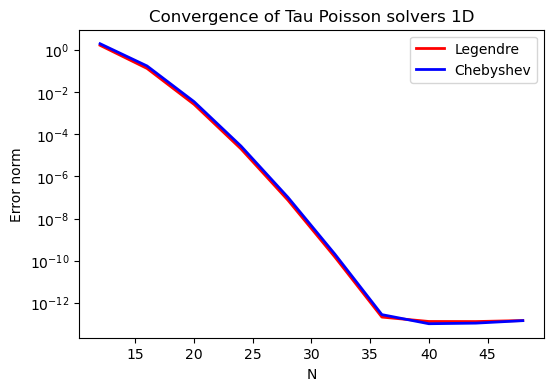
The spectral convergence is evident and we can see that after \(N=40\) roundoff errors dominate as the errornorm trails off around \(10^{-14}\).

Complete solver

A complete solver, that can use either Legendre or Chebyshev bases, chosen as a command-line argument, can also be found here.