Demo - Sparse Chebyshev-Petrov-Galerkin methods for differentiation
Mikael Mortensen (email: mikaem@math.uio.no), Department of Mathematics, University of Oslo.
Date: October 26, 2021
Summary. This demo explores how to use sparse Chebyshev-Petrov-Galerkin methods for finding Chebyshev coefficients of the derivatives of smooth functions. We will compare the methods to the more commonly adopted recursion methods that are found in most spectral textbooks.
Introduction
The Chebyshev polynomials of the first kind can be defined as
where \(\theta = \cos^{-1} x\), \(k\) is a positive integer and \(x \in [-1, 1]\). The Chebyshev polynomials span the discrete space \(S_N = \text{span}\{T_k\}_{k=0}^{N-1}\), and a function \(u(x)\) can be approximated in this space as
Consider the expansion of the function \(u(x)=\sin(\pi x)\), created in shenfun as
from shenfun import *
import sympy as sp
x = sp.Symbol('x')
ue = sp.sin(sp.pi*x)
N = 16
SN = FunctionSpace(N, 'C')
uN = Function(SN, buffer=ue)
uN
Function([-2.08166817e-17,  5.69230686e-01, -1.58270808e-16,
          -6.66916672e-01,  5.37523027e-17,  1.04282369e-01,
          -4.62011417e-17, -6.84063354e-03, -1.96261557e-17,
           2.50006885e-04, -3.39031315e-18, -5.85024831e-06,
          -7.53729275e-17,  9.53478051e-08, -6.47840243e-17,
          -1.15621280e-09])
The Python Function uN represents the expansion (2), and the printed
values represent \(\boldsymbol{\hat{u}} = \{\hat{u}_k\}_{k=0}^{N-1}\). The expansion is fairly well resolved since
the highest values of \(\{\hat{u}_k\}_{k=0}^{N-1}\) approach 0.
Note that the coefficients obtained are based on interpolation at
quadrature points and they do not agree completely with the coefficients truncated from an
infinite series \(u(x) = \sum_{k=0}^{\infty} \hat{u}_k T_k\). The obtained series is
often denoted as \(u_N(x) = I_N u(x)\), where \(I_N\) is an interpolation operator.
Under the hood the coefficients are found by projection using quadrature for the integrals:
find \(u_N \in S_N\) such that
where \(\omega = (1-x^2)\) and the scalar product notation
\((a, b)_{\omega^{-1/2}} = \sum_{j=0}^{N-1} a(x_j)b(x_j)\omega_j \approx \int_{-1}^{1} a(x)b(x) \omega(x)^{-1/2} dx\),
where \(\{\omega_j\}_{j=0}^{N-1}\) are the quadrature weights. The quadrature approach ensures
that \(u(x_j) = u_N(x_j)\) for all quadrature points \(\{x_j\}_{j=0}^{N-1}\).
In shenfun we compute the following under the hood: insert for \(u_N = \sum_{j=0}^{N-1} \hat{u}_j T_j\),
\(u=\sin(\pi x)\) and \(v = T_k\) to get
This has now become a linear algebra problem, and we recognise the matrix \(d^{(0)}_{kj} = (T_j, T_k)_{\omega^{-1/2}}=c_k \pi /2 \delta_{kj}\), where \(\delta_{kj}\) is the Kronecker delta function, and \(c_0=2\) and \(c_k=1\) for \(k>0\). The problem is solved trivially since \(d^{(0)}_{kj}\) is diagonal, and thus
where \(I^N = \{0, 1, \ldots, N-1\}\). We can compare this to the truncated coefficients, where the integral \((\sin(\pi x), T_k)_{\omega^{-1/2}}\) is computed with high precision. To this end we could use adaptive quadrature, or symbolic integration with sympy, but it is sufficient to use a large enough number of polynomials to fully resolve the function. Below we find this number to be 22 and we see that the absolute error in the highest wavenumber \(\hat{u}_{15} \approx 10^{-11}\).
SM = FunctionSpace(0, 'C')
uM = Function(SM, buffer=ue, abstol=1e-16, reltol=1e-16)
print(uM[:N] - uN[:N])
print(len(uM))
[-9.46212805e-18  1.11022302e-16 -2.47551551e-18 -1.11022302e-16
  2.58329282e-17  0.00000000e+00  7.16473371e-17 -1.74339709e-16
  3.25619527e-18 -8.74951153e-17  4.95408707e-17  4.56246674e-16
  1.45411069e-16 -7.76002561e-14  9.02561799e-17  1.05743319e-11]
22
Differentiation
Let us now consider the \(n\)’th derivative of \(u(x)\) instead, denoted here as \(u^{(n)}\). We want to find \(u^{(n)}\) in the space \(S_N\), which means that we want to obtain the following expansion
First note that this expansion is not the same as the derivative of the previously found \(u_N\), which is
where \(T^{(n)}_k\) is the \(n\)’th derivative of \(T_k\), a polynomial of order \(k-n\). We again use projection to find \(u_N^{(n)} \in S_N\) such that
Inserting for \(u_N^{(n)}\) and \(u^{(n)} = (u_N)^{(n)}\) we get
where \(d^{(n)}_{kj} = (T_j^{(n)}, T_k)_{\omega^{-1/2}}\). We compute \(\hat{u}_k^{(n)}\) by inverting the diagonal \(d^{(0)}_{kj}\)
The matrix \(d^{(n)}_{kj}\) is upper triangular, and the last \(n\) rows are zero. Since \(d^{(n)}_{kj}\) is dense the matrix vector product \(\sum_{j=0}^{N-1} d^{(n)}_{kj} \hat{u}_j\) is costly and also susceptible to roundoff errors if the structure of the matrix is not taken advantage of. But computing it in shenfun is straightforward, for \(n=1\) and \(2\):
uN1 = project(Dx(uN, 0, 1), SN)
uN2 = project(Dx(uN, 0, 2), SN)
uN1
Function([-9.55804991e-01, -4.76220620e-15, -3.05007135e+00,
          -4.12912297e-15,  9.51428681e-01, -4.55914139e-15,
          -9.13950067e-02, -4.00472769e-15,  4.37386282e-03,
          -3.69070920e-15, -1.26261106e-04, -3.62290294e-15,
           2.44435655e-06, -1.81395268e-15, -3.46863840e-08,
           0.00000000e+00])
where uN1 \(=u_N^{(1)}\) and uN2 \(=u_N^{(2)}\).
Alternatively, doing all the work that goes on under the hood
u = TrialFunction(SN)
v = TestFunction(SN)
D0 = inner(u, v)
D1 = inner(Dx(u, 0, 1), v)
D2 = inner(Dx(u, 0, 2), v)
w0 = Function(SN) # work array
uN1 = Function(SN)
uN2 = Function(SN)
uN1 = D0.solve(D1.matvec(uN, w0), uN1)
uN2 = D0.solve(D2.matvec(uN, w0), uN2)
uN1
Function([-9.55804991e-01, -4.76220620e-15, -3.05007135e+00,
          -4.12912297e-15,  9.51428681e-01, -4.55914139e-15,
          -9.13950067e-02, -4.00472769e-15,  4.37386282e-03,
          -3.69070920e-15, -1.26261106e-04, -3.62290294e-15,
           2.44435655e-06, -1.81395268e-15, -3.46863840e-08,
           0.00000000e+00])
We can look at the sparsity patterns of \((d^{(1)}_{kj})\) and \((d^{(2)}_{kj})\)
%matplotlib inline

import matplotlib.pyplot as plt
fig, (ax1, ax2) = plt.subplots(1, 2)
ax1.spy(D1.diags(), markersize=2, color='r')
ax2.spy(D2.diags(), markersize=2, color='b')
<matplotlib.lines.Line2D at 0x163fb2660>
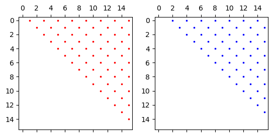
just to see that they are upper triangular. We now ask is there a better and faster
way to get uN1 and uN2? A better approach would involve only sparse
matrices, like the diagonal \((d^{(0)}_{kj})\). But how do we get there?
Most textbooks on spectral methods use fast recursive methods to
find the coefficients \(\{\hat{u}_k^{(n)}\}\). Here we will show a fast Galerkin approach.
It turns out that a simple change of test space/function will be sufficient. Let us first replace the test space \(S_N\) with the Dirichlet space \(D_N=\{v \in S_N | v(\pm 1) = 0\}\) using basis functions \(v=T_k-T_{k+2}\) and see what happens. Because of the two boundary conditions, the number of degrees of freedom is reduced by two, and we need to use a space with \(N+2\) quadrature points in order to get a square matrix system. The method now becomes classified as Chebyshev-Petrov-Galerkin, as we wish to find \(u_N^{(1)} \in S_N\) such that
The implementation is straightforward
DN = FunctionSpace(N+2, 'C', bc=(0, 0))
v = TestFunction(DN)
D0 = inner(u, v)
D1 = inner(Dx(u, 0, 1), v)
uN11 = Function(SN)
uN11 = D0.solve(D1.matvec(uN, w0), uN11)
print(uN11-uN1)
[2.22044605e-16 7.88860905e-31 8.88178420e-16 0.00000000e+00
 0.00000000e+00 0.00000000e+00 0.00000000e+00 0.00000000e+00
 0.00000000e+00 0.00000000e+00 2.71050543e-20 0.00000000e+00
 4.23516474e-22 0.00000000e+00 0.00000000e+00 0.00000000e+00]
and since uN11 = uN1 we see that we have achived the same result as in
the regular projection. However, the matrices in use now look like
fig, (ax1, ax2) = plt.subplots(1, 2)
ax1.spy(D0.diags(), markersize=2, color='r')
ax2.spy(D1.diags(), markersize=2, color='b')
<matplotlib.lines.Line2D at 0x167eb5880>
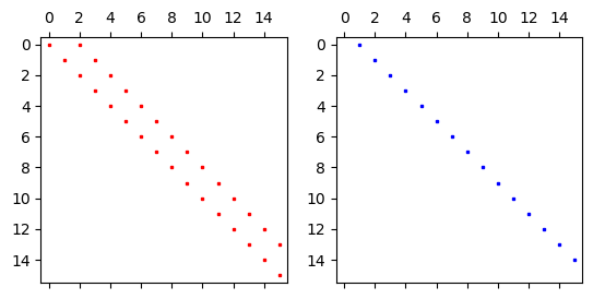
So \((d^{(0)}_{kj})\) now contains two nonzero diagonals, whereas \((d^{(1)}_{kj})\) is
a matrix with one single diagonal. There is no longer a full differentiation
matrix, and we can easily perform this projection for millions of degrees of freedom.
What about \((d^{(2)}_{kj})\)? We can now use biharmonic test functions that
satisfy four boundary conditions in the space \(B_N = \{v \in S_N | v(\pm 1) = v'(\pm 1) =0\}\),
and continue in a similar fashion:
BN = FunctionSpace(N+4, 'C', bc=(0, 0, 0, 0))
v = TestFunction(BN)
D0 = inner(u, v)
D2 = inner(Dx(u, 0, 2), v)
uN22 = Function(SN)
uN22 = D0.solve(D2.matvec(uN, w0), uN22)
print(uN22-uN2)
[-4.38649204e-12 -2.01002713e+00 -4.16887590e-12  1.53351702e-01
 -1.65264542e-12 -6.03926282e-03 -5.52731678e-13  1.47222317e-04
 -1.25657449e-13 -2.61304093e-06  2.52435490e-29  6.77626358e-21
  0.00000000e+00  6.35274710e-22  0.00000000e+00  0.00000000e+00]
We get that uN22 = uN2, so the Chebyshev-Petrov-Galerkin projection works. The matrices involved are now
fig, (ax1, ax2) = plt.subplots(1, 2)
ax1.spy(D0.diags(), markersize=2, color='r')
ax2.spy(D2.diags(), markersize=2, color='b')
<matplotlib.lines.Line2D at 0x163fb31d0>
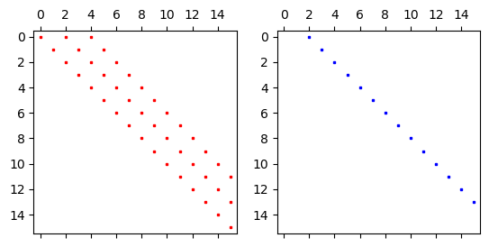
So there are now three nonzero diagonals in \((d^{(0)}_{kj})\), whereas the differentiation matrix \((d^{(2)}_{kj})\) contains only one nonzero diagonal.
Why does this work so well? The Chebyshev polynomials and their derivatives satisfy the following orthogonality relation
where
So when we choose a test function \(\omega^n T^{(n)}_k\) and a trial function \(T_j\), we get the diagonal differentiation matrix
The two chosen test functions above are both proportional to \(\omega^n T^{(n)}_k\). More precisely, \(T_k-T_{k+2} = \frac{2}{k+1} \omega T^{(1)}_{k+1}\) and the biharmonic test function is \(T_k-\frac{2(k+2)}{k+3}T_{k+2} + \frac{k+1}{k+3}T_{k+4} = \frac{4 \omega^2T^{(2)}_{k+2}}{(k+2)(k+3)}\). Using these very specific test functions correponds closely to using the Chebyshev recursion formulas that are found in most textbooks. Here they are adapted to a Chebyshev-Petrov-Galerkin method, where we simply choose test and trial functions and everything else falls into place in a few lines of code.
Recursion
Let us for completion show how to find \(\hat{u}_N^{(1)}\) with a recursive approach. The Chebyshev polynomials satisfy
By using this and setting \(u' = \sum_{k=0}^{\infty} \hat{u}^{(1)}_k T_k = \sum_{k=0}^{\infty} \hat{u}_k T'_k\) we get
Using this recursion on a discrete series, together with \(\hat{u}^{(1)}_{N} = \hat{u}^{(1)}_{N-1} = 0\), we get (see [canuto] Eq. (2.4.24))
which is easily implemented in a (slow) for-loop
f1 = np.zeros(N+1)
ck = np.ones(N); ck[0] = 2
for k in range(N-2, -1, -1):
    f1[k] = (f1[k+2]+2*(k+1)*uN[k+1])/ck[k]
print(f1[:-1]-uN1)
[ 0.00000000e+00  0.00000000e+00  4.44089210e-16  0.00000000e+00
 -1.11022302e-16  0.00000000e+00 -1.38777878e-17  0.00000000e+00
  0.00000000e+00  0.00000000e+00  0.00000000e+00  0.00000000e+00
  0.00000000e+00  0.00000000e+00  0.00000000e+00  0.00000000e+00]
which evidently is exactly the same result. It turns out that this is not strange. If we multiply (11) by \(\pi/2\), rearrange a little bit and move to a matrix form we get
which is exactly how \(\boldsymbol{\hat{u}^{(1)}}\) was computed above with the Chebyshev-Petrov-Galerkin approach
(compare with the code line uN11 = D0.solve(D1.matvec(uN, w0), uN11)). Not convinced? Check that the matrices
D0 and D1 are truly as stated above. The matrices below are printed as dictionaries with diagonal
number as key (main is 0, first upper is 1 etc) and diagonal values as values:
import pprint
DN = FunctionSpace(N+2, 'C', bc=(0, 0))
v = TestFunction(DN)
D0 = inner(u, v)
D1 = inner(Dx(u, 0, 1), v)
pprint.pprint(dict(D0))
pprint.pprint(dict(D1))
{0: array([3.14159265, 1.57079633, 1.57079633, 1.57079633, 1.57079633,
       1.57079633, 1.57079633, 1.57079633, 1.57079633, 1.57079633,
       1.57079633, 1.57079633, 1.57079633, 1.57079633, 1.57079633,
       1.57079633]),
 2: array([-1.57079633, -1.57079633, -1.57079633, -1.57079633, -1.57079633,
       -1.57079633, -1.57079633, -1.57079633, -1.57079633, -1.57079633,
       -1.57079633, -1.57079633, -1.57079633, -1.57079633])}
{1: array([ 3.14159265,  6.28318531,  9.42477796, 12.56637061, 15.70796327,
       18.84955592, 21.99114858, 25.13274123, 28.27433388, 31.41592654,
       34.55751919, 37.69911184, 40.8407045 , 43.98229715, 47.1238898 ,
       50.26548246])}
In conclusion, we have shown that we can use an efficient Chebyshev-Petrov-Galerkin approach to obtain the discrete Chebyshev coefficients for the derivatives of a function. By inspection, it turns out that this approach is identical to the common methods based on well-known Chebyshev recursion formulas.