Demo - Helmholtz equation in polar coordinates

Authors:

Mikael Mortensen (mikaem at math.uio.no)

Date:

April 8, 2020

Summary. This is a demonstration of how the Python module shenfun can be used to solve the Helmholtz equation on a circular disc, using polar coordinates. This demo is implemented in a single Python file unitdisc_helmholtz.py, and the numerical method is described in more detail by J. Shen [She97].

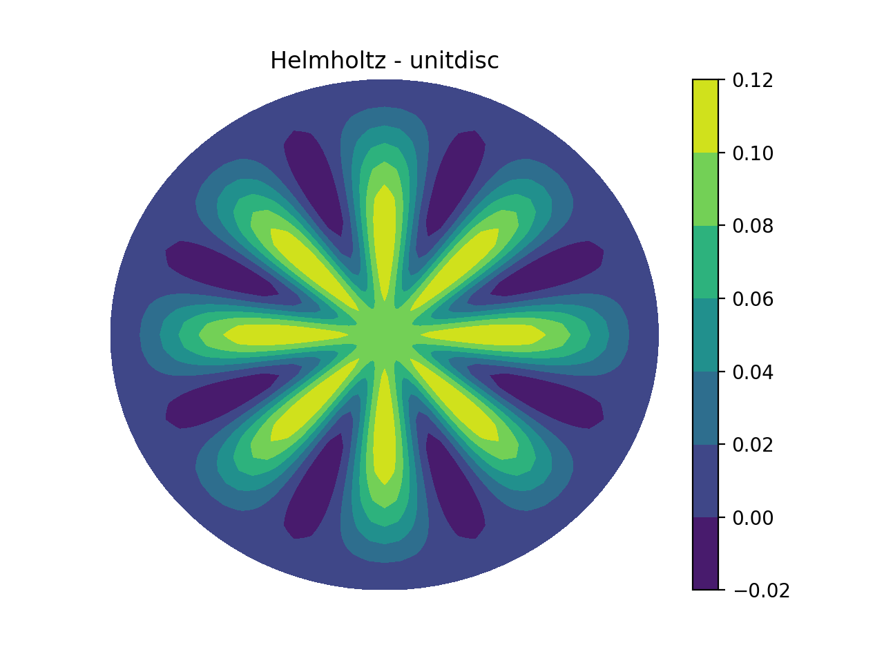
Helmholtz on the unit disc

Helmholtz equation

The Helmholtz equation is given as

(1)\[ -\nabla^2 u(\boldsymbol{x}) + \alpha u(\boldsymbol{x}) = f(\boldsymbol{x}) \quad \text{for }\, \boldsymbol{x}=(x, y) \in \Omega,\]

(2)\[ u =0 \text{ on } \partial \Omega,\]

where \(u(\boldsymbol{x})\) is the solution, \(f(\boldsymbol{x})\) is a function and \(\alpha\) a constant. The domain is a circular disc \(\Omega = \{(x, y): x^2+y^2 < a^2\}\) with radius \(a\). We use polar coordinates \((\theta, r)\), defined as

(3)\[ x = r \cos \theta,\]

(4)\[ y = r \sin \theta,\]

which leads to a Cartesian product mesh \((\theta, r) \in [0, 2\pi) \times [0, a]\) suitable for numerical implementations. Note that the two directions are ordered with \(\theta\) first and then \(r\), which is less common than \((r, \theta)\). This has to do with the fact that we will need to solve linear equation systems along the radial direction, but not the \(\theta\)-direction, since Fourier matrices are diagonal. When the radial direction is placed last, the data in the radial direction will be contigeous in a row-major C memory, leading to faster memory access where it is needed the most. Note that it takes very few changes in shenfun to switch the directions to \((r, \theta)\) if this is still desired.

We will use Chebyshev or Legendre basis functions \(\psi_j(r)\) for the radial direction and a periodic Fourier expansion in \(\exp(\imath k \theta)\) for the azimuthal direction. The polar basis functions are as such

(5)\[ v_{kj}(\theta, r) = \exp(\imath k \theta) \psi_j(r),\]

and we look for solutions

(6)\[ u(\mathbf{x}) = \tilde{u}(\theta, r) = \sum_{k} \sum_{j} \hat{u}_{kj} v_{kj}(\theta, r).\]

Note that \(\tilde{u}\) is the function \(u\) mapped to computational space. From now on we will simply use \(u(\theta, r)\) without the tilde, and assume that the proper version of the function is understood from its arguments.

A discrete Fourier approximation space with \(N\) basis functions is then

(7)\[ V_F^N = \text{span} \{\exp(\imath k \theta)| \text{ for } k \in K\},\]

where the index set \(K = \{-N/2, -N/2+1, \ldots, N/2-1\}\). Since the solution \(u(\theta, r)\) is real, there is Hermitian symmetry and \(\hat{u}_{k,j} = \hat{u}_{k,-j}^*\) (with \(*\) denoting a complex conjugate). For this reason we use only \(k \in K=\{0, 1, \ldots, N/2\}\) in solving for \(\hat{u}_{kj}\), and then use Hermitian symmetry to get the remaining unknowns.

The radial basis is more tricky, because there is a nontrivial ‘boundary’ condition (pole condition) that needs to be applied at the center of the disc \((r=0)\)

(8)\[ \frac{\partial u(\theta, 0)}{\partial \theta} = 0.\]

To apply this condition we split the solution into Fourier coefficients with wavenumber 0 and \(K\backslash \{0\}\), remembering that the Fourier basis function with \(k=0\) is simply 1

(9)\[ u(\theta, r) = \sum_{j} \left( \hat{u}_{0j} \psi_{j}(r) + \sum_{k=1}^{N/2} \hat{u}_{kj} \exp(\imath k \theta) \psi_j(r) \right).\]

We then apply a different radial basis for the two \(\psi\)’s in the above equation (renaming the first \(\overline{\psi}\))

(10)\[ u(\theta, r) = \sum_{j} \left( \hat{u}_{0j} \overline{\psi}_{j}(r) + \sum_{k=1}^{N/2} \hat{u}_{kj} \exp(\imath k \theta) \psi_j(r) \right).\]

Note that the first term \(\sum_{j} \hat{u}_{0j} \overline{\psi}_{j}(r)\) is independent of \(\theta\). Now, to enforce conditions

(11)\[ u(\theta, a) = 0,\]

(12)\[ \frac{\partial u(\theta, 0)}{\partial \theta} = 0,\]

it is sufficient for the two bases (\(\overline{\psi}\) and \(\psi\)) to satisfy

(13)\[ \overline{\psi}_j(a) = 0,\]

(14)\[ \psi_j(a) = 0,\]

(15)\[ \psi_j(0) = 0.\]

Bases that satisfy these conditions can be found both with Legendre and Chebyshev polynomials. If \(\phi_j(x)\) is used for either the Legendre polynomial \(L_j(x)\) or the Chebyshev polynomial of the first kind \(T_j(x)\), we can have

(16)\[ \overline{\psi}_j(r) = \phi_j(2r/a-1) - \phi_{j+1}(2r/a-1), \text{ for } j \in 0, 1, \ldots N-1,\]

(17)\[ \psi_j(r) = \phi_j(2r/a-1) - \phi_{j+2}(2r/a-1), \text{ for } j \in 0, 1, \ldots N-2.\]

Define the following approximation spaces for the radial direction

(18)\[ V_D^N = \text{span} \{\psi_j\}_{j=0}^{N-3}\]

(19)\[ V_U^N = \text{span} \{\overline{\psi}_j\}_{j=0}^{N-2}\]

(20)\[\]

and split the function space for the azimuthal direction into

(21)\[ V_F^0 = \text{span}\{1\},\]

(22)\[ V_F^{1} = \text{span} \{\exp(\imath k \theta)\}, \text{ for } k \in K \backslash \{0\}.\]

We then look for solutions

(23)\[ u(\theta, r) = u^0(r) + u^1(\theta, r),\]

where

(24)\[ u^0(r) = \sum_{j=0}^{N-2} \hat{u}^0_j \overline{\psi}_j(r),\]

(25)\[ u^1(\theta, r) = \sum_{j=0}^{N-3}\sum_{k=1}^{N/2} \hat{u}^1_{kj} \exp(\imath k \theta) \psi_j(r) .\]

As such the Helmholtz problem is split in two smaller problems. The two problems read with the spectral Galerkin method:

Find \(u^0 \in V_F^0 \otimes V_U^N\) such that

(26)\[ \int_{\Omega} (-\nabla^2 u^0 + \alpha u^0) v^0 w d\sigma = \int_{\Omega} f v^0 w d\sigma, \quad \forall \, v^0 \in V_F^0 \otimes V_U^N.\]

Find \(u^1 \in V_F^1 \otimes V_D^N\) such that

(27)\[ \int_{\Omega} (-\nabla^2 u^1 + \alpha u^1) v^1 w d\sigma = \int_{\Omega} f v^1 w d\sigma, \quad \forall \, v^1 \in V_F^1 \otimes V_D^N.\]

Note that integration over the domain is done using polar coordinates with an integral measure of \(d\sigma=rdrd\theta\). However, the integral in the radial direction needs to be mapped to \(t=2r/a-1\), where \(t \in [-1, 1]\), which suits the basis functions used, see (17). This leads to a measure of \(0.5(t+1)adtd\theta\). Furthermore, the weight \(w(t)\) will be unity for the Legendre basis and \((1-t^2)^{-0.5}\) for the Chebyshev bases.

Implementation

A complete implementation is found in the file unitdisc_helmholtz.py. Here we give a brief explanation for the implementation. Start by importing all functionality from shenfun and sympy, where Sympy is required for handeling the polar coordinates. Also, we choose to work with covariant basis vectors.

from shenfun import *
import sympy as sp
config['basisvectors'] = 'covariant'

# Define polar coordinates using angle along first axis and radius second
theta, r = psi = sp.symbols('x,y', real=True, positive=True)
rv = (r*sp.cos(theta), r*sp.sin(theta)) # Map to Cartesian (x, y)

Note that Sympy symbols are both positive and real, \(\theta\) is chosen to be along the first axis and \(r\) second. This has to agree with the next step, which is the creation of tensorproductspaces \(V_F^0 \otimes V_U^N\) and \(V_F^1 \otimes V_D^N\). We use domain=(0, 1) for the radial direction to get a unit disc, whereas the default domain for the Fourier bases is already the required \((0, 2\pi)\).

N = 32
F = FunctionSpace(N, 'F', dtype='d')
F0 = FunctionSpace(1, 'F', dtype='d')
L = FunctionSpace(N, 'L', bc=(0, 0), domain=(0, 1))
L0 = FunctionSpace(N, 'L', bc=(None, 0), domain=(0, 1))
T = TensorProductSpace(comm, (F, L), axes=(1, 0), coordinates=(psi, rv))
T0 = TensorProductSpace(MPI.COMM_SELF, (F0, L0), axes=(1, 0), coordinates=(psi, rv))

Note that since F0 only has one component we could actually use L0 without creating T0. But the code turns out to be simpler if we use T0, much because the additional \(\theta\)-direction is required for the polar coordinates to apply. Using one single basis function for the \(\theta\) direction is as such a generic way to handle polar 1D problems (i.e., problems that are only functions of the radial direction, but still using polar coordinates). Also note that F is created using the entire range of wavenumbers even though it should not include wavenumber 0. As such we need to make sure that the coefficient created for \(k=0\) (i.e., \(\hat{u}^1_{0,j}\)) will be exactly zero. Finally, note that T0 is not distributed with MPI, which is accomplished using MPI.COMM_SELF instead of comm (which equals MPI.COMM_WORLD). The purely radial problem (26) is only solved on the one processor with rank = 0.

Polar coordinates are ensured by feeding coordinates=(psi, rv) to TensorProductSpace. Operators like div() grad() and curl() will now work on items of Function, TestFunction and TrialFunction using a polar coordinate system.

To define the equations (26) and (27) we first declare these test- and trialfunctions, and then use code that is remarkably similar to the mathematics.

v = TestFunction(T)
u = TrialFunction(T)
v0 = TestFunction(T0)
u0 = TrialFunction(T0)
alpha = 1

mats = inner(v, -div(grad(u))+alpha*u)
if comm.Get_rank() == 0:
    mats0 = inner(v0, -div(grad(u0))+alpha*u0)

Here mats and mats0 will contain several tensor product matrices in the form of TPMatrix. Since there is only one non-periodic direction the matrices can be easily solved using la.SolverGeneric1ND. But first we need to define the function \(f(\theta, r)\). To this end we use sympy and the method of manufactured solution to define a possible solution ue, and then compute f exactly using exact differentiation

# Manufactured solution
ue = (r*(1-r))**2*sp.cos(8*theta)-0.1*(r-1)
#f = -ue.diff(r, 2) - (1/r)*ue.diff(r, 1) - (1/r**2)*ue.diff(theta, 2) + alpha*ue
f = (-div(grad(u))+alpha*u).tosympy(basis=ue, psi=psi)

# Compute the right hand side on the quadrature mesh
fj = Array(T, buffer=f)

# Take scalar product
f_hat = Function(T)
f_hat = inner(v, fj, output_array=f_hat)
if T.local_slice(True)[0].start == 0: # The processor that owns k=0
    f_hat[0] = 0

# For k=0 we solve only a 1D equation. Do the scalar product for Fourier
# coefficient 0 by hand (or sympy).
if comm.Get_rank() == 0:
    f0_hat = Function(T0)
    gt = sp.lambdify(r, sp.integrate(f, (theta, 0, 2*sp.pi))/2/sp.pi)(L0.mesh())
    f0_hat = T0.scalar_product(gt, f0_hat)

Note that for \(u^0\) we perform the interal in the \(\theta\) direction exactly using sympy. This is necessary since one Fourier coefficient is not sufficient to do this integral numerically. For the \(u^1\) case we do the integral numerically as part of the inner() product. With the correct right hand side assembled we can solve the linear system of equations

u_hat = Function(T)
Sol1 = la.SolverGeneric1ND(mats)
u_hat = Sol1(f_hat, u_hat)

# case k = 0
u0_hat = Function(T0)
if comm.Get_rank() == 0:
    Sol0 = la.SolverGeneric1ND(mats0)
    u0_hat = Sol0(f0_hat, u0_hat)
comm.Bcast(u0_hat, root=0)

Having found the solution in spectral space all that is left is to transform it back to real space.

# Transform back to real space. Broadcast 1D solution
sl = T.local_slice(False)
uj = u_hat.backward() + u0_hat.backward()[:, sl[1]]

Postprocessing

The solution can now be compared with the exact solution through

uq = Array(T, buffer=ue)
print('Error =', np.linalg.norm(uj-uq))

We can also get the gradient of the solution. For this we need a space without boundary conditions, and a vector space

TT = T.get_orthogonal()
V = VectorSpace(TT)

Notice that we do not have the solution in one single space in spectral space, since it is a combination of u_hat and u0_hat. For this reason we first transform the solution from real space uj to the new orthogonal space TT

ua = Array(TT, buffer=uj)
uh = ua.forward()

With the solution as a Function we can simply project the gradient to V

dv = project(grad(uh), V)
du = dv.backward()

Note that the gradient du now contains the contravariant components of the covariant basis vector b. The basis vector b is not normalized (it’s length is not unity), because we have set config['basisvectors']='covariant'. The basisvectors can be seen as

from IPython.display import Math
Math(T.coors.latex_basis_vectors(symbol_names={theta: '\\theta', r: 'r'}))

and we see that they are given in terms of the Cartesian unit vectors. The gradient we have computed is (and yes, it should be \(r^2\) because we do not have unit vectors)

(28)\[ \nabla u = \underbrace{\frac{1}{r^2}\frac{\partial u}{\partial \theta}}_{du[0]}\mathbf{b}_{\theta} + \underbrace{\frac{\partial u}{\partial r}}_{du[1]} \mathbf{b}_{r}\]

Now it makes sense to plot the solution and its gradient in Cartesian instead of computational coordinates. To this end we need to project the gradient to a Cartesian basis

\[\begin{split}\begin{align*} \frac{\partial u}{\partial x} &= \nabla u \cdot \mathbf{i},\\ \frac{\partial u}{\partial y} &= \nabla u \cdot \mathbf{j}. \end{align*}\end{split}\]

We compute the Cartesian gradient by assembling (28) on the computational grid

ui, vi = TT.local_mesh(True)
b = T.coors.get_covariant_basis()
bij = np.array(sp.lambdify(psi, b)(ui, vi))
gradu = du[0]*bij[0] + du[1]*bij[1]

Because of the way the vectors are stored, gradu[0] will now contain \(\nabla u \cdot \mathbf{i}\) and gradu[1] will contain \(\nabla u \cdot \mathbf{j}\).

To validate the gradient we compute the \(L^2\) error norm

\[\sqrt{\int_{\Omega} |\nabla u - \nabla u_e|^2 d\sigma} = \sqrt{\int_{\theta=0}^{2\pi}\int_{r=0}^{1} \left(\left(\frac{1}{r^2}\frac{\partial u-u_e}{\partial \theta}\right)^2\mathbf{b}_{\theta}\cdot \mathbf{b}_{\theta} + \left(\frac{\partial u-u_e}{\partial r}\right)^2\mathbf{b}_{r}\cdot \mathbf{b}_{r} \right)rd\theta dr}\]

implemented as

gradue = Array(V, buffer=grad(u).tosympy(basis=ue, psi=psi))
gij = T.coors.get_covariant_metric_tensor()
ui, vi = TT.local_mesh(True, kind='uniform')
# Evaluate metric on computational mesh
g = np.array(sp.lambdify(psi, gij)(ui, vi), dtype=object)
# Compute L2 error
errorg = inner(1, (du[0]-gradue[0])**2*g[0, 0]+ (du[1]-gradue[1])**2*g[1, 1])
print('Error gradient', np.sqrt(errorg))

Error gradient 5.577949e-12

We now refine the solution to make it look better, and plot on the unit disc.

u_hat2 = u_hat.refine([N*3, N*3])
u0_hat2 = u0_hat.refine([1, N*3])
sl = u_hat2.function_space().local_slice(False)
ur = u_hat2.backward() + u0_hat2.backward()[:, sl[1]]

# Wrap periodic plot around since it looks nicer
xx, yy = u_hat2.function_space().local_cartesian_mesh()
xp = np.vstack([xx, xx[0]])
yp = np.vstack([yy, yy[0]])
up = np.vstack([ur, ur[0]])
# For vector no need to wrap around and no need to refine:
xi, yi = TT.local_cartesian_mesh()

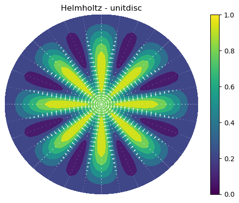
# plot
import matplotlib.pyplot as plt
plt.figure()
plt.contourf(xp, yp, up)
plt.quiver(xi, yi, gradu[0], gradu[1], scale=40, pivot='mid', color='white')
plt.colorbar()
plt.title('Helmholtz - unitdisc')
plt.xticks([])
plt.yticks([])
plt.axis('off')
plt.show()

Solution of Helmholtz equation, with gradient