Demo - Kuramato-Sivashinsky equation
Mikael Mortensen (email: mikaem@math.uio.no), Department of Mathematics, University of Oslo.
Date: April 13, 2018
Summary. This is a demonstration of how the Python module shenfun can be used to solve the time-dependent, nonlinear Kuramato-Sivashinsky equation, in a doubly periodic domain. The demo is implemented in a single Python file KuramatoSivashinsky.py, and it may be run in parallel using MPI.
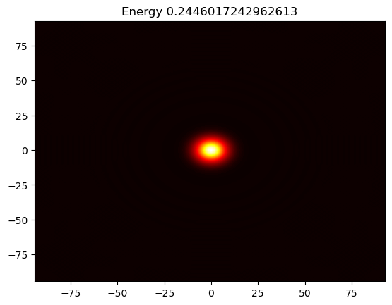
Figure 1: Movie showing the evolution of the solution of the Kuramato-Sivashinsky equation.
The Kuramato-Sivashinsky equation
The Kuramato-Sivashinsky (KS) equation is known for its chaotic bahaviour, and it is often used in study of turbulence or turbulent combustion. We will here solve the KS equation in a doubly periodic domain \(\Omega=[-30\pi, 30\pi)^2\), starting from a single Gaussian pulse
Spectral Galerkin method
The PDE in (1) can be solved with many different numerical methods. We will here use the shenfun software and this software makes use of the spectral Galerkin method. Being a Galerkin method, we need to reshape the governing equations into proper variational forms, and this is done by multiplying (1) with the complex conjugate of a proper test function and then integrating over the domain. To this end we use testfunction \(v\in W^N(\Omega)\), where \(W^N(\Omega)\) is a suitable function space (defined in Eq. (7)), and obtain
Note that the overline is used to indicate a complex conjugate, whereas \(w\) is a weight function. The function \(u\) is now to be considered a trial function, and the integrals over the domain are often referred to as inner products. With inner product notation
the variational problem can be formulated as
The space and time discretizations are still left open. There are numerous different approaches that one could take for discretizing in time. Here we will use a fourth order exponential Runge-Kutta method.
Discretization
We discretize the model equation in space using continuously differentiable Fourier basis functions
where \(l\) is the wavenumber, and \(\underline{l}=\frac{2\pi}{L}l\) is the scaled wavenumber, scaled with domain length \(L\) (here \(60\pi\)). Since we want to solve these equations on a computer, we need to choose a finite number of test functions. A discrete function space \(V^N\) can be defined as
where \(N\) is chosen as an even positive integer and \(\boldsymbol{l} = (-N/2, -N/2+1, \ldots, N/2-1)\). And now, since \(\Omega\) is a two-dimensional domain, we can create a tensor product of two such one-dimensional spaces:
where \(\boldsymbol{N} = (N, N)\). Obviously, it is not necessary to use the same number (\(N\)) of basis functions for each direction, but it is done here for simplicity. A 2D tensor product basis function is now defined as
where the indices for \(y\)-direction are \(\underline{m}=\frac{2\pi}{L}m\), and \(\boldsymbol{m}\) is the same set as \(\boldsymbol{l}\) due to using the same number of basis functions for each direction. One distinction, though, is that for the \(y\)-direction expansion coefficients are only stored for \(m=(0, 1, \ldots, N/2)\) due to Hermitian symmetry (real input data).
We now look for solutions of the form
The expansion coefficients \(\hat{u}_{lm}\) can be related directly to the solution \(u(x, y)\) using Fast Fourier Transforms (FFTs) if we are satisfied with obtaining the solution in quadrature points corresponding to
Note that these points are different from the standard (like \(2\pi j/N\)) since the domain is set to \([-30\pi, 30\pi]^2\) and not the more common \([0, 2\pi]^2\). We now have
where \(\boldsymbol{u} = \{u(x_i, y_j)\}_{(i,j)\in \boldsymbol{i} \times \boldsymbol{j}}\), \(\boldsymbol{\hat{u}} = \{\hat{u}_{lm}\}_{(l,m)\in \boldsymbol{l} \times \boldsymbol{m}}\) and \(\mathcal{F}_x^{-1}\) is the inverse Fourier transform along direction \(x\), for all indices in the other direction. Note that the two inverse FFTs are performed sequentially, one direction at the time, and that there is no scaling factor due the definition used for the inverse Fourier transform:
Note that this differs from the definition used by, e.g., Numpy.
The inner products used in Eq. (4) may be computed using forward FFTs (using weight functions \(w=1/L\)):
From this we see that the variational forms may be written in terms of the Fourier transformed \(\hat{u}\). Expanding the exact derivatives of the nabla operator, we have
where the indices on the right hand side run over \(\boldsymbol{l} \times \boldsymbol{m}\). We find that the equation to be solved for each wavenumber can be found directly as
Implementation
The model equation (1) is implemented in shenfun using Fourier basis functions for both \(x\) and \(y\) directions. We start the solver by implementing necessary functionality from required modules like Numpy, Sympy and matplotlib, in addition to shenfun:
from sympy import symbols, exp, lambdify
import numpy as np
import matplotlib.pyplot as plt
import time
from shenfun import *
The size of the problem (in real space) is then specified, before creating
the TensorProductSpace, which is using a tensor product of two
one-dimensional Fourier function spaces. We also
create a VectorSpace, since this is required for computing the
gradient of the scalar field u. The gradient is required for the nonlinear
term.
# Size of discretization
N = (128, 128)

K0 = FunctionSpace(N[0], 'F', domain=(-30*np.pi, 30*np.pi), dtype='D')
K1 = FunctionSpace(N[1], 'F', domain=(-30*np.pi, 30*np.pi), dtype='d')
T = TensorProductSpace(comm, (K0, K1), **{'planner_effort': 'FFTW_MEASURE'})
TV = VectorSpace([T, T])
Tp = T.get_dealiased((1.5, 1.5))
TVp = VectorSpace(Tp)
Test and trialfunctions are required for assembling the variational forms:
u = TrialFunction(T)
v = TestFunction(T)
and some arrays are required to hold the solution. We also create an array
gradu, that will be used to compute the gradient in the nonlinear term.
Finally, the wavenumbers are collected in an array K. Here one feature is worth
mentioning. The gradient in spectral space can be computed as 1j*K*U_hat.
However, since this is an odd derivative, and we are using an even number N
for the size of the domain, the highest wavenumber must be set to zero. This is
the purpose of the last keyword argument to local_wavenumbers below.
x, y = symbols("x,y", real=True)
ue = exp(-0.01*(x**2+y**2))
U = Array(T, buffer=ue)
U_hat = Function(T)
U_hat = U.forward(U_hat)
mask = T.get_mask_nyquist()
U_hat.mask_nyquist(mask)
gradu = Array(TVp)
K = np.array(T.local_wavenumbers(True, True, eliminate_highest_freq=True))
X = T.local_mesh(True)
Note that using this K in computing derivatives has the same effect as
achieved by symmetrizing the Fourier series by replacing the first sum below
with the second when computing odd derivatives.
Here \(\sideset{}{'}\sum\) means that the first and last items in the sum are divided by two. Note that the two sums are equal as they stand (due to aliasing), but only the latter (known as the Fourier interpolant) gives the correct (zero) derivative of the basis with the highest wavenumber.
Shenfun has a few integrators implemented in the shenfun.utilities.integrators
submodule. Two such integrators are the 4th order explicit Runge-Kutta method
RK4, and the exponential 4th order Runge-Kutta method ETDRK4. Both these
integrators need two methods provided by the problem being solved, representing
the linear and nonlinear terms in the problem equation. We define two methods
below, called LinearRHS and NonlinearRHS
def LinearRHS(self, u,**params):
    # Assemble diagonal bilinear forms
    return -(div(grad(u))+div(grad(div(grad(u)))))

def NonlinearRHS(self, U, U_hat, dU, gradu, **params):
    # Assemble nonlinear term
    gradu = TVp.backward(1j*K*U_hat, gradu)
    dU = Tp.forward(0.5*(gradu[0]*gradu[0]+gradu[1]*gradu[1]), dU)
    dU.mask_nyquist(mask)
    dU *= -1
    return dU
The code should, hopefully, be self-explanatory.
All that remains now is to setup the integrator plus some plotting functionality for visualizing the results. Note that visualization is only nice when running the code in serial. For parallel, it is recommended to use HDF5File, to store intermediate results to the HDF5 format, for later viewing in, e.g., Paraview.
We create an update function for plotting intermediate results with a cool colormap:
from IPython.display import display

# Integrate using an exponential time integrator
def update(self, u, u_hat, t, tstep, **params):
    if tstep % params['plot_step'] == 0 and params['plot_step'] > 0:
        u = u_hat.backward(u)
        self.image = plt.contourf(X[0], X[1], u, 256, cmap=plt.get_cmap('hot'))
        self.image.axes.set_title(f'Energy {dx(u**2)}')
        display(self.image, clear=True)
        plt.pause(1e-6)
Now all that remains is to create the integrator and call it
par = {'plot_step': 100, 'gradu': gradu}
dt = 0.01
end_time = 10
integrator = ETDRK4(T, L=LinearRHS, N=NonlinearRHS, update=update, image=None, **par)
#integrator = RK4(T, L=LinearRHS, N=NonlinearRHS, update=update, **par)
integrator.setup(dt)
U_hat = integrator.solve(U, U_hat, dt, (0, end_time))
<matplotlib.contour.QuadContourSet at 0x7fc0155f4050>