Demo - 1D Poisson’s equation
Mikael Mortensen (email: mikaem@math.uio.no), Department of Mathematics, University of Oslo.
Date: April 13, 2018
Summary. This is a demonstration of how the Python module shenfun can be used to solve Poisson’s equation with Dirichlet boundary conditions in one dimension. Spectral convergence, as shown in the figure below, is demonstrated. The demo is implemented in slightly more generic terms (more boundary conditions) in poisson1D.py, and the numerical method is is described in more detail by J. Shen [She94] and [She95].
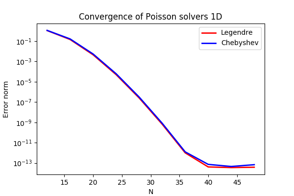
Figure 1: Convergence of 1D Poisson solvers for both Legendre and Chebyshev modified basis function.
Poisson’s equation
Poisson’s equation is given as
where \(u(x)\) is the solution, \(f(x)\) is a function and \(a, b\) are two possibly non-zero constants.
To solve Eq. (1) with the Galerkin method we need smooth continuously differentiable basis functions, \(v_k\), that satisfy the given boundary conditions. And then we look for solutions like
where \(N\) is the size of the discretized problem, \(\{\hat{u}_k\}_{k=0}^{N-1}\) are the unknown expansion coefficients, and the function space is \(\text{span}\{v_k\}_{k=0}^{N-1}\).
The basis functions of the function space can, for example, be constructed from Chebyshev, \(T_k(x)\), or Legendre, \(L_k(x)\), polynomials and we use the common notation \(\phi_k(x)\) to represent either one of them. It turns out that it is easiest to use basis functions with homogeneous Dirichlet boundary conditions
for \(k=0, 1, \ldots N-3\). This gives the function space \(V^N_0 = \text{span}\{v_k(x)\}_{k=0}^{N-3}\). We can then add two more linear basis functions (that belong to the kernel of Poisson’s equation)
which gives the inhomogeneous space \(V^N = \text{span}\{v_k\}_{k=0}^{N-1}\). With the two linear basis functions it is easy to see that the last two degrees of freedom, \(\hat{u}_{N-2}\) and \(\hat{u}_{N-1}\), now are given as
and, as such, we only have to solve for \(\{\hat{u}_k\}_{k=0}^{N-3}\), just like for a problem with homogeneous boundary conditions (for homogeneous boundary condition we simply have \(\hat{u}_{N-2} = \hat{u}_{N-1} = 0\)). We now formulate a variational problem using the Galerkin method: Find \(u \in V^N\) such that
Note that since we only have \(N-3\) unknowns we are only using the homogeneous test functions from \(V^N_0\).
The weighted integrals, weighted by \(w(x)\), are called inner products, and a common notation is
The integral can either be computed exactly, or with quadrature. The advantage of the latter is that it is generally faster, and that non-linear terms may be computed just as quickly as linear. For a linear problem, it does not make much of a difference, if any at all. Approximating the integral with quadrature, we obtain
where \(\{w_j\}_{j=0}^{N-1}\) are quadrature weights. The quadrature points \(\{x_j\}_{j=0}^{N-1}\) are specific to the chosen basis, and even within basis there are two different choices based on which quadrature rule is selected, either Gauss or Gauss-Lobatto.
Inserting for test and trialfunctions, we get the following bilinear form and matrix \(A=(a_{jk})\in\mathbb{R}^{N-2\times N-2}\) for the Laplacian
Note that the sum runs over \(k=0, 1, \ldots, N-3\) since the second derivatives of \(v_{N-2}\) and \(v_{N-1}\) are zero. The right hand side linear form and vector is computed as \(\tilde{f}_j = (f, v_j)_w^N\), for \(j=0,1,\ldots, N-3\), where a tilde is used because this is not a complete transform of the function \(f\), but only an inner product.
By defining the column vectors \(\boldsymbol{\hat{u}}=(\hat{u}_0, \hat{u}_1, \ldots, \hat{u}_{N-3})^T\) and \(\boldsymbol{\tilde{f}}=(\tilde{f}_0, \tilde{f}_1, \ldots, \tilde{f}_{N-3})^T\) we get the linear system of equations
Now, when the expansion coefficients \(\boldsymbol{\hat{u}}\) are found by solving this linear system, they may be transformed to real space \(u(x)\) using (3), and here the contributions from \(\hat{u}_{N-2}\) and \(\hat{u}_{N-1}\) must be accounted for. Note that the matrix \(A\) (different for Legendre or Chebyshev) has a very special structure that allows for a solution to be found very efficiently in order of \(\mathcal{O}(N)\) operations, see [She94] and [She95]. These solvers are implemented in shenfun for both bases.
Method of manufactured solutions
In this demo we will use the method of manufactured
solutions to demonstrate spectral accuracy of the shenfun Dirichlet bases. To
this end we choose an analytical function that satisfies the given boundary
conditions:
where \(k\) is an integer and \(a\) and \(b\) are constants. Now, feeding \(u_e\) through the Laplace operator, we see that the last two linear terms disappear, whereas the first term results in
Now, setting \(f_e(x) = \nabla^2 u_e(x)\) and solving for \(\nabla^2 u(x) = f_e(x)\), we can compare the numerical solution \(u(x)\) with the analytical solution \(u_e(x)\) and compute error norms.
Implementation
Preamble
We will solve Poisson’s equation using the shenfun Python module. The first thing needed is then to import some of this module’s functionality plus some other helper modules, like Numpy and Sympy:
from shenfun import inner, div, grad, TestFunction, TrialFunction, Function, \
    project, Dx, Array, FunctionSpace, dx
import numpy as np
from sympy import symbols, cos, sin, exp, lambdify
We use Sympy for the manufactured solution and Numpy for testing.
Manufactured solution
The exact solution \(u_e(x)\) and the right hand side \(f_e(x)\) are created using
Sympy as follows
a = -1
b = 1
k = 4
x = symbols("x")
ue = sin(k*np.pi*x)*(1-x**2) + a*(1 - x)/2. + b*(1 + x)/2.
fe = ue.diff(x, 2)
These solutions are now valid for a continuous domain. The next step is thus to discretize, using a discrete mesh \(\{x_j\}_{j=0}^{N-1}\) and a finite number of basis functions.
Note that it is not mandatory to use Sympy for the manufactured solution. Since the
solution is known (14), we could just as well simply use Numpy
to compute \(f_e\) at \(\{x_j\}_{j=0}^{N-1}\). However, with Sympy it is much
easier to experiment and quickly change the solution.
Discretization
We create a basis with a given number of basis functions, and extract the computational mesh from the basis itself
N = 32
SD = FunctionSpace(N, 'Chebyshev', bc=(a, b))
#SD = FunctionSpace(N, 'Legendre', bc=(a, b))
Note that we can either choose a Legendre or a Chebyshev basis.
Variational formulation
The variational problem (9) can be assembled using shenfun’s
TrialFunction, TestFunction and inner() functions.
u = TrialFunction(SD)
v = TestFunction(SD)
# Assemble left hand side matrix
A = inner(v, div(grad(u)))
# Assemble right hand side
fj = Array(SD, buffer=fe)
f_hat = Function(SD)
f_hat = inner(v, fj, output_array=f_hat)
/home/docs/checkouts/readthedocs.org/user_builds/shenfun/conda/latest/lib/python3.13/site-packages/shenfun/matrixbase.py:171: FutureWarning: Input has data type int64, but the output has been cast to float64.  In the future, the output data type will match the input. To avoid this warning, set the `dtype` parameter to `None` to have the output dtype match the input, or set it to the desired output data type.
  self._diags = sp_diags(list(self.values()),
Note that the sympy function fe can be used to initialize the Array
fj. We wrap this Numpy array in an Array class
(fj = Array(SD, buffer=fe)), because an Array
is required as input to the inner() function.
Solve linear equations
Finally, solve linear equation system and transform solution from spectral
\(\boldsymbol{\hat{u}}\) vector to the real space \(\{u(x_j)\}_{j=0}^{N-1}\)
and then check how the solution corresponds with the exact solution \(u_e\).
To this end we compute the \(L_2\)-errornorm using the shenfun function
dx()
u_hat = A.solve(f_hat)
uj = SD.backward(u_hat)
ua = Array(SD, buffer=ue)
print("Error=%2.16e" %(np.sqrt(dx((uj-ua)**2))))
Error=2.3565353252967906e-10
Convergence test
To do a convergence test we will now create a function main, that takes the
number of quadrature points as parameter, and prints out
the error.
def main(N, family='Chebyshev'):
    SD = FunctionSpace(N, family=family, bc=(a, b))
    u = TrialFunction(SD)
    v = TestFunction(SD)

    # Get f on quad points
    fj = Array(SD, buffer=fe)

    # Compute right hand side of Poisson's equation
    f_hat = Function(SD)
    f_hat = inner(v, fj, output_array=f_hat)

    # Get left hand side of Poisson's equation
    A = inner(v, div(grad(u)))

    f_hat = A.solve(f_hat)
    uj = SD.backward(f_hat)

    # Compare with analytical solution
    ua = Array(SD, buffer=ue)
    l2_error = np.linalg.norm(uj-ua)
    return l2_error
For example, we find the error of a Chebyshev discretization using 12 quadrature points as
main(12, 'Chebyshev')
np.float64(1.1654916318123927)
To get the convergence we call main for a list
of \(N=[12, 16, \ldots, 48]\), and collect the errornorms in
arrays to be plotted. The error can be plotted using
matplotlib, and the generated
figure is also shown in this demos summary.
%matplotlib inline

import matplotlib.pyplot as plt

N = range(12, 50, 4)
error = {}
for basis in ('legendre', 'chebyshev'):
    error[basis] = []
    for i in range(len(N)):
        errN = main(N[i], basis)
        error[basis].append(errN)

plt.figure(figsize=(6, 4))
for basis, col in zip(('legendre', 'chebyshev'), ('r', 'b')):
    plt.semilogy(N, error[basis], col, linewidth=2)
plt.title('Convergence of Poisson solvers 1D')
plt.xlabel('N')
plt.ylabel('Error norm')
plt.legend(('Legendre', 'Chebyshev'))
plt.show()
/home/docs/checkouts/readthedocs.org/user_builds/shenfun/conda/latest/lib/python3.13/site-packages/shenfun/matrixbase.py:171: FutureWarning: Input has data type int64, but the output has been cast to float64.  In the future, the output data type will match the input. To avoid this warning, set the `dtype` parameter to `None` to have the output dtype match the input, or set it to the desired output data type.
  self._diags = sp_diags(list(self.values()),
The spectral convergence is evident and we can see that after \(N=40\) roundoff errors dominate as the errornorm trails off around \(10^{-14}\).
Complete solver
A complete solver, that can use any family of bases (Chebyshev, Legendre, Jacobi, Chebyshev second kind), and any kind of boundary condition, can be found here.
J. Shen. Efficient Spectral-Galerkin Method I. Direct Solvers of Second- and Fourth-Order Equations Using Legendre Polynomials, SIAM Journal on Scientific Computing, 15(6), pp. 1489-1505, doi: 10.1137/0915089, 1994.
J. Shen. Efficient Spectral-Galerkin Method II. Direct Solvers of Second- and Fourth-Order Equations Using Chebyshev Polynomials, SIAM Journal on Scientific Computing, 16(1), pp. 74-87, doi: 10.1137/0916006, 1995.