Demo - Helmholtz equation on the unit sphere
Mikael Mortensen (email: mikaem@math.uio.no), Department of Mathematics, University of Oslo.
Date: April 20, 2020
Summary. This is a demonstration of how the Python module shenfun can be used to solve the Helmholtz equation on a unit sphere, using spherical coordinates. This demo is implemented in a single Python file sphere_helmholtz.py. If requested the solver will run in parallel using MPI.
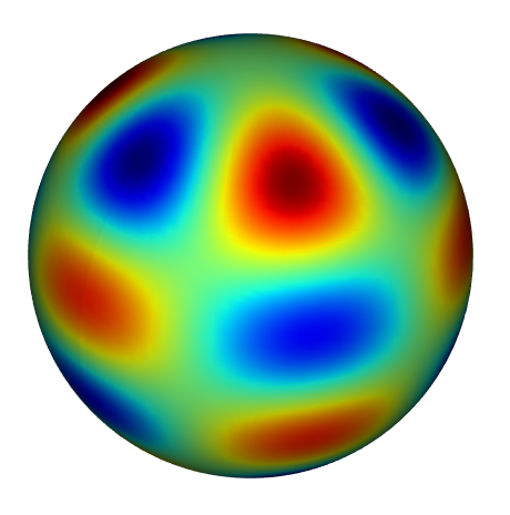
Figure 1: Helmholtz on the unit sphere.
Helmholtz equation
The Helmholtz equation is given as
where \(u(\boldsymbol{x})\) is the solution, \(f(\boldsymbol{x})\) is a function and \(\alpha\) a constant. We use spherical coordinates \((\theta, \phi)\), defined as
which (with \(r=1\)) leads to a 2D Cartesian product mesh \((\theta, \phi) \in (0, \pi) \times [0, 2\pi)\) suitable for numerical implementations. There are no boundary conditions on the problem under consideration. However, with the chosen Cartesian mesh, periodic boundary conditions are required for the \(\phi\)-direction. As such, the \(\phi\)-direction will use a Fourier basis \(\exp(\imath k \phi)\).
A regular Chebyshev or Legendre basis \(\psi_j(\theta) = \gamma_j(2\theta/\pi-1)\) will be used for the \(\theta\)-direction, where \(\gamma_j\) could be either the Chebyshev polynomial of first kind \(T_j\) or the Legendre polynomial \(L_j\). Note the mapping from real coordinates \(\theta\) to computational coordinates in domain \([-1, 1]\).
The spherical basis functions are as such
and we look for solutions
A discrete Fourier approximation space with \(N\) basis functions is then
where the index set \(K = \{-N/2, -N/2+1, \ldots, N/2-1\}\). For this demo we assume that the solution is complex, and as such there is no simplification possible for Hermitian symmetry.
The following approximation space is used for the \(\theta\)-direction
and the variational formulation of the problem reads: find \(u \in V^N \otimes V_F^N\) such that
Note that integration over the domain is done using spherical coordinates with an integral measure of \(d\sigma=\sin \theta d\theta d\phi\).
Implementation
A complete implementation is found in the file sphere_helmholtz.py. Here we give a brief explanation for the implementation. Start by importing all functionality from shenfun and sympy, where Sympy is required for handeling the spherical coordinates.
from shenfun import *
import sympy as sp

# Define spherical coordinates with unit radius
r = 1
theta, phi = sp.symbols('x,y', real=True, positive=True)
psi = (theta, phi)
rv = (r*sp.sin(theta)*sp.cos(phi), r*sp.sin(theta)*sp.sin(phi), r*sp.cos(theta))
Note that the position vector rv has three components (for \((x, y, z)\))
even though the computational domain is only 2D.
Also note that Sympy symbols are both positive and real, and \(\theta\) is
chosen to be along the first axis and \(\phi\) second. This has to agree with
the next step, which is the creation of tensorproductspaces
\(V^N \otimes V_F^N\).
N, M = 40, 30
L0 = FunctionSpace(N, 'C', domain=(0, np.pi))
F1 = FunctionSpace(M, 'F', dtype='D')
T = TensorProductSpace(comm, (L0, F1), coordinates=(psi, rv, sp.Q.positive(sp.sin(theta))))
Spherical coordinates are ensured by feeding coordinates=(psi, rv, sp.Q.positive(sp.sin(theta)))
to TensorProductSpace, where the restriction sp.Q.positive(sp.sin(theta)) is there
to help sympy. Operators like div(),
grad() and curl() will now work on
items of Function, TestFunction and
TrialFunction using a spherical coordinate system.
To define the equation (6) we first declare these test- and trialfunctions, and then use code that is very similar to the mathematics.
alpha = 2
v = TestFunction(T)
u = TrialFunction(T)
mats = inner(v, -div(grad(u))+alpha*u)
Here mats will be a list containing several tensor product
matrices in the form of
TPMatrix. Since there is only one directions with
non-diagonal matrices (\(\theta\)-direction) we
can use the generic SolverGeneric1ND solver.
Note that some of the non-diagonal matrices will be dense,
which is a weakness of the current method. Also note
that with Legendre one can use integration by parts
instead
        mats = inner(grad(v), grad(u))
        mats += [inner(v, alpha*u)]
To solve the problem we also need to define the function \(f(\theta, r)\).
To this end we use sympy and the method of
manufactured solution to define a possible solution ue,
and then compute f exactly using exact differentiation. We use
the spherical harmonics function
to define an analytical solution
alpha = 2
sph = sp.functions.special.spherical_harmonics.Ynm
ue = sph(6, 3, theta, phi)

# Compute the right hand side on the quadrature mesh
# That is, compute f = -div(grad(ue)) + alpha*ue
f = (-div(grad(u))+alpha*u).tosympy(basis=ue, psi=psi)
fj = Array(T, buffer=f)

# Take scalar product
f_hat = Function(T)
f_hat = inner(v, fj, output_array=f_hat)

u_hat = Function(T)
Sol = la.SolverGeneric1ND(mats)
u_hat = Sol(f_hat, u_hat)
Having found the solution in spectral space all that is left is to transform it back to real space.
uj = u_hat.backward()
uq = Array(T, buffer=ue)
print('Error =', np.linalg.norm(uj-uq))
Error = 3.828188771680728e-12
Postprocessing
We can refine the solution to make it look better, and plot on the unit sphere using either mayavi or plotly using the shenfun function surf3D().
u_hat2 = u_hat.refine([N*2, M*2])
fig = surf3D(u_hat2.backward().real, wrapaxes=[1])
fig.show()