Demo - Lid driven cavity

Authors:

Mikael Mortensen (mikaem at math.uio.no)

Date:

May 6, 2019

Summary. The lid driven cavity is a classical benchmark for Navier Stokes solvers. This is a demonstration of how the Python module shenfun can be used to solve the lid driven cavity problem with full spectral accuracy using a mixed (coupled) basis in a 2D tensor product domain. The demo also shows how to use mixed tensor product spaces for vector valued equations. Note that the regular lid driven cavity, where the top wall has constant velocity and the remaining three walls are stationary, has a singularity at the two upper corners, where the velocity is discontinuous. Due to their global nature, spectral methods are usually not very good at handling problems with discontinuities, and for this reason we will also look at a regularized lid driven cavity, where the top lid moves according to \((1-x)^2(1+x)^2\), thus removing the corner discontinuities.

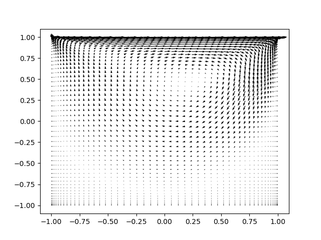
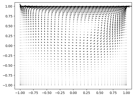
Velocity vectors for the lid driven cavity at Reynolds number 100

Navier Stokes equations

The nonlinear steady Navier Stokes equations are given in strong form as

\[\begin{split}\begin{align*} \nu \nabla^2 \boldsymbol{u} - \nabla p &= \nabla \cdot \boldsymbol{u} \boldsymbol{u} \quad \text{in } \Omega , \\ \nabla \cdot \boldsymbol{u} &= 0 \quad \text{in } \Omega, \\ \int_{\Omega} p dx &= 0, \\ \boldsymbol{u}(x, y=1) = (1, 0) \, &\text{ or }\, \boldsymbol{u}(x, y=1) = ((1-x)^2(1+x)^2, 0), \\ \boldsymbol{u}(x, y=-1) &= (0, 0), \\ \boldsymbol{u}(x=\pm 1, y) &= (0, 0), \end{align*}\end{split}\]

where \(\boldsymbol{u}, p\) and \(\nu\) are, respectively, the fluid velocity vector, pressure and kinematic viscosity. The domain \(\Omega = (-1, 1)^2\) and the nonlinear term \(\boldsymbol{u} \boldsymbol{u}\) is the outer product of vector \(\boldsymbol{u}\) with itself. Note that the final \(\int_{\Omega} p dx = 0\) is there because there is no Dirichlet boundary condition on the pressure and the system of equations would otherwise be ill conditioned.

We want to solve these steady nonlinear Navier Stokes equations with the Galerkin method, using the shenfun Python package. The first thing we need to do then is to import all of shenfun’s functionality

import matplotlib.pyplot as plt
from shenfun import *

Note that MPI for Python (mpi4py) is a requirement for shenfun, but the current solver cannot be used with more than one processor.

Tensor product spaces

With the Galerkin method we need function spaces for both velocity and pressure, as well as for the nonlinear right hand side. A Dirichlet space will be used for velocity, whereas there is no boundary restriction on the pressure space. For both two-dimensional spaces we will use one basis function for the \(x\)-direction, \(\mathcal{X}_k(x)\), and one for the \(y\)-direction, \(\mathcal{Y}_l(y)\). And then we create two-dimensional basis functions like

(1)\[ v_{kl}(x, y) = \mathcal{X}_k(x) \mathcal{Y}_l(y),\]

and solutions (trial functions) as

(2)\[ u(x, y) = \sum_{k}\sum_{l} \hat{u}_{kl} v_{kl}(x, y).\]

For the homogeneous Dirichlet boundary condition the basis functions \(\mathcal{X}_k(x)\) and \(\mathcal{Y}_l(y)\) are chosen as composite Legendre polynomials (we could also use Chebyshev):

(3)\[ \mathcal{X}_k(x) = L_k(x) - L_{k+2}(x), \quad \forall \, k \in \boldsymbol{k}^{N_0-2},\]

(4)\[ \mathcal{Y}_l(y) = L_l(y) - L_{l+2}(y), \quad \forall \, l \in \boldsymbol{l}^{N_1-2},\]

where \(\boldsymbol{k}^{N_0-2} = (0, 1, \ldots, N_0-3)\), \(\boldsymbol{l}^{N_1-2} = (0, 1, \ldots, N_1-3)\) and \(N = (N_0, N_1)\) is the number of quadrature points in each direction. Note that \(N_0\) and \(N_1\) do not need to be the same. The basis funciton (3) satisfies the homogeneous Dirichlet boundary conditions at \(x=\pm 1\) and (4) the same at \(y=\pm 1\). As such, the basis function \(v_{kl}(x, y)\) satisfies the homogeneous Dirichlet boundary condition for the entire domain.

With shenfun we create these homogeneous spaces, \(D_0^{N_0}(x)=\text{span}\{L_k-L_{k+2}\}_{k=0}^{N_0-2}\) and \(D_0^{N_1}(y)=\text{span}\{L_l-L_{l+2}\}_{l=0}^{N_1-2}\) as

N = (45, 45)
family = 'Legendre' # or use 'Chebyshev'
quad = 'GL'         # for Chebyshev use 'GC' or 'GL'
D0X = FunctionSpace(N[0], family, quad=quad, bc=(0, 0))
D0Y = FunctionSpace(N[1], family, quad=quad, bc=(0, 0))

The spaces are here the same, but we will use D0X in the \(x\)-direction and D0Y in the \(y\)-direction. But before we use these bases in tensor product spaces, they remain identical as long as \(N_0 = N_1\).

Special attention is required by the moving lid. To get a solution with nonzero boundary condition at \(y=1\) we need to add one more basis function that satisfies that solution. In general, a nonzero boundary condition can be added on both sides of the domain using the following basis

(5)\[ \mathcal{Y}_l(y) = L_l(y) - L_{l+2}(y), \quad \forall \, l \in \boldsymbol{l}^{N_1-2}.\]

(6)\[ \mathcal{Y}_{N_1-2}(y) = (L_0+L_1)/2 \quad \left(=(1+y)/2\right),\]

(7)\[ \mathcal{Y}_{N_1-1}(y) = (L_0-L_1)/2 \quad \left(=(1-y)/2\right).\]

And then the unknown component \(N_1-2\) decides the value at \(y=1\), whereas the unknown at \(N_1-1\) decides the value at \(y=-1\). Here we only need to add the \(N_1-2\) component, but for generality this is implemented in shenfun using both additional basis functions. We create the space \(D_1^{N_1}(y)=\text{span}\{\mathcal{Y}_l(y)\}_{l=0}^{N_1-1}\) as

D1Y = FunctionSpace(N[1], family, quad=quad, bc=(0, 1))

where bc=(0, 1) fixes the values for \(y=-1\) and \(y=1\), respectively. For a regularized lid driven cavity the velocity of the top lid is \((1-x)^2(1+x)^2\) and not unity. To implement this boundary condition instead, we can make use of sympy and quite straight forward do

import sympy
x = sympy.symbols('x')
#D1Y = FunctionSpace(N[1], family, quad=quad, bc=(0, (1-x)**2*(1+x)**2))

Uncomment the last line to run the regularized boundary conditions. Otherwise, there is no difference at all between the regular and the regularized lid driven cavity implementations.

The pressure basis that comes with no restrictions for the boundary is a little trickier. The reason for this has to do with inf-sup stability. The obvious choice of basis functions are the regular Legendre polynomials \(L_k(x)\) in \(x\) and \(L_l(y)\) in the \(y\)-directions. The problem is that for the natural choice of \((k, l) \in \boldsymbol{k}^{N_0} \times \boldsymbol{l}^{N_1}\) there are nullspaces and the problem is not well-defined. It turns out that the proper choice for the pressure basis is simply the regular Legendre basis functions, but for \((k, l) \in \boldsymbol{k}^{N_0-2} \times \boldsymbol{l}^{N_1-2}\). The bases \(P^{N_0}(x)=\text{span}\{L_k(x)\}_{k=0}^{N_0-3}\) and \(P^{N_1}(y)=\text{span}\{L_l(y)\}_{l=0}^{N_1-3}\) are created as

PX = FunctionSpace(N[0], family, quad=quad)
PY = FunctionSpace(N[1], family, quad=quad)
PX.slice = lambda: slice(0, N[0]-2)
PY.slice = lambda: slice(0, N[1]-2)

Note that we still use these spaces with the same \(N_0 \cdot N_1\) quadrature points in real space, but the two highest frequencies have been set to zero.

We have now created all relevant function spaces for the problem at hand. It remains to combine these spaces into tensor product spaces, and to combine tensor product spaces into mixed (coupled) tensor product spaces. From the Dirichlet bases we create two different tensor product spaces, whereas one is enough for the pressure

(8)\[ V_{1}^{\boldsymbol{N}}(\boldsymbol{x}) = D_0^{N_0}(x) \otimes D_1^{N_1}(y),\]

(9)\[ V_{0}^{\boldsymbol{N}}(\boldsymbol{x}) = D_0^{N_0}(x) \otimes D_0^{N_1}(y),\]

(10)\[ P^{\boldsymbol{N}}(\boldsymbol{x}) = P^{N_0}(x) \otimes P^{N_1}(y).\]

With shenfun the tensor product spaces are created as

V1 = TensorProductSpace(comm, (D0X, D1Y))
V0 = TensorProductSpace(comm, (D0X, D0Y))
P = TensorProductSpace(comm, (PX, PY), modify_spaces_inplace=True)

where modify_spaces_inplace=True makes use of PX and PY directly. These spaces have now been modified to fit in the TensorProductSpace P, along two different directions and as such the original spaces have been modified. The default behavior in shenfun is to make copies of the 1D spaces under the hood, and thus leave PX and PY untouched. In that case the two new and modified spaces would be accessible from P.bases.

Note that all these tensor product spaces are scalar valued. The velocity is a vector, and a vector requires a mixed vector basis like \(W_1^{\boldsymbol{N}} = V_1^{\boldsymbol{N}} \times V_0^{\boldsymbol{N}}\). The vector basis is created in shenfun as

W1 = VectorSpace([V1, V0])
W0 = VectorSpace([V0, V0])

Note that the second vector basis, \(W_0^{\boldsymbol{N}} = V_0^{\boldsymbol{N}} \times V_0^{\boldsymbol{N}}\), uses homogeneous boundary conditions throughout.

Mixed variational form

We now formulate a variational problem using the Galerkin method: Find \(\boldsymbol{u} \in W_1^{\boldsymbol{N}}\) and \(p \in P^{\boldsymbol{N}}\) such that

(11)\[ \int_{\Omega} (\nu \nabla^2 \boldsymbol{u} - \nabla p ) \cdot \boldsymbol{v} \, dxdy = \int_{\Omega} (\nabla \cdot \boldsymbol{u}\boldsymbol{u}) \cdot \boldsymbol{v}\, dxdy \quad\forall \boldsymbol{v} \, \in \, W_0^{\boldsymbol{N}},\]

(12)\[ \int_{\Omega} \nabla \cdot \boldsymbol{u} \, q \, dxdy = 0 \quad\forall q \, \in \, P^{\boldsymbol{N}}.\]

Note that we are using test functions \(\boldsymbol{v}\) with homogeneous boundary conditions.

The first obvious issue with Eq (11) is the nonlinearity. In other words we will need to linearize and iterate to be able to solve these equations with the Galerkin method. To this end we will introduce the solution on iteration \(k \in [0, 1, \ldots]\) as \(\boldsymbol{u}^k\) and compute the nonlinearity using only known solutions \(\int_{\Omega} (\nabla \cdot \boldsymbol{u}^k\boldsymbol{u}^k) \cdot \boldsymbol{v}\, dxdy\). Using further integration by parts we end up with the equations to solve for iteration number \(k+1\) (using \(\boldsymbol{u} = \boldsymbol{u}^{k+1}\) and \(p=p^{k+1}\) for simplicity)

(13)\[ -\int_{\Omega} \nu \nabla \boldsymbol{u} \, \colon \nabla \boldsymbol{v} \, dxdy + \int_{\Omega} p \nabla \cdot \boldsymbol{v} \, dxdy = \int_{\Omega} (\nabla \cdot \boldsymbol{u}^k\boldsymbol{u}^k) \cdot \boldsymbol{v}\, dxdy \quad\forall \boldsymbol{v} \, \in \, W_0^{\boldsymbol{N}},\]

(14)\[ \int_{\Omega} \nabla \cdot \boldsymbol{u} \, q \, dxdy = 0 \quad\forall q \, \in \, P^{\boldsymbol{N}}.\]

Note that the nonlinear term may also be integrated by parts and evaluated as \(\int_{\Omega}-\boldsymbol{u}^k\boldsymbol{u}^k \, \colon \nabla \boldsymbol{v} \, dxdy\). All boundary integrals disappear since we are using test functions with homogeneous boundary conditions.

Since we are to solve for \(\boldsymbol{u}\) and \(p\) at the same time, we formulate a mixed (coupled) problem: find \((\boldsymbol{u}, p) \in W_1^{\boldsymbol{N}} \times P^{\boldsymbol{N}}\) such that

(15)\[ a((\boldsymbol{u}, p), (\boldsymbol{v}, q)) = L((\boldsymbol{v}, q)) \quad \forall (\boldsymbol{v}, q) \in W_0^{\boldsymbol{N}} \times P^{\boldsymbol{N}},\]

where bilinear (\(a\)) and linear (\(L\)) forms are given as

(16)\[ a((\boldsymbol{u}, p), (\boldsymbol{v}, q)) = -\int_{\Omega} \nu \nabla \boldsymbol{u} \, \colon \nabla \boldsymbol{v} \, dxdy + \int_{\Omega} p \nabla \cdot \boldsymbol{v} \, dxdy + \int_{\Omega} \nabla \cdot \boldsymbol{u} \, q \, dxdy,\]

(17)\[ L((\boldsymbol{v}, q); \boldsymbol{u}^{k}) = \int_{\Omega} (\nabla \cdot \boldsymbol{u}^{k}\boldsymbol{u}^{k}) \cdot \boldsymbol{v}\, dxdy.\]

Note that the bilinear form will assemble to a block matrix, whereas the right hand side linear form will assemble to a block vector. The bilinear form does not change with the solution and as such it does not need to be reassembled inside an iteration loop.

The algorithm used to solve the equations are:

• Set \(k = 0\)

• Guess \(\boldsymbol{u}^0 = (0, 0)\)

• while not converged:

  • assemble \(L((\boldsymbol{v}, q); \boldsymbol{u}^{k})\)

  • solve \(a((\boldsymbol{u}, p), (\boldsymbol{v}, q)) = L((\boldsymbol{v}, q); \boldsymbol{u}^{k})\) for \(\boldsymbol{u}^{k+1}, p^{k+1}\)

  • compute error = \(\int_{\Omega} (\boldsymbol{u}^{k+1}-\boldsymbol{u}^{k})^2 \, dxdy\)

  • if error \(<\) some tolerance then converged = True

  • \(k\) += \(1\)

Implementation of solver

We will now implement the coupled variational problem described in previous sections. First of all, since we want to solve for the velocity and pressure in a coupled solver, we have to create a mixed tensor product space \(VQ = W_1^{\boldsymbol{N}} \times P^{\boldsymbol{N}}\) that couples velocity and pressure

VQ = CompositeSpace([W1, P])    # Coupling velocity and pressure

We can now create test- and trialfunctions for the coupled space \(VQ\), and then split them up into components afterwards:

up = TrialFunction(VQ)
vq = TestFunction(VQ)
u, p = up
v, q = vq

Note

The test function v is using homogeneous Dirichlet boundary conditions even though it is derived from VQ, which contains W1. It is currently not (and will probably never be) possible to use test functions with inhomogeneous boundary conditions.

With the basisfunctions in place we may assemble the different blocks of the final coefficient matrix. For this we also need to specify the kinematic viscosity, which is given here in terms of the Reynolds number:

Re = 100.
nu = 2./Re
if family.lower() == 'legendre':
    A = inner(grad(v), -nu*grad(u))
    G = inner(div(v), p)
else:
    A = inner(v, nu*div(grad(u)))
    G = inner(v, -grad(p))
D = inner(q, div(u))

The assembled subsystems A, G and D are lists containg the different blocks of the complete, coupled, coefficient matrix. A actually contains 4 tensor product matrices of type TPMatrix. The first two matrices are for vector component zero of the test function v[0] and trial function u[0], the matrices 2 and 3 are for components 1. The first two matrices are as such for

A[0:2] = inner(grad(v[0]), -nu*grad(u[0]))

Breaking it down the inner product is mathematically

(18)\[ \int_{\Omega}-\nu \left(\frac{\partial \boldsymbol{v}[0]}{\partial x}, \frac{\partial \boldsymbol{v}[0]}{\partial y}\right) \cdot \left(\frac{\partial \boldsymbol{u}[0]}{\partial x}, \frac{\partial \boldsymbol{u}[0]}{\partial y}\right) dx dy .\]

We can now insert for test function \(\boldsymbol{v}[0]\)

(19)\[ \boldsymbol{v}[0]_{kl} = \mathcal{X}_k \mathcal{Y}_l, \quad (k, l) \in \boldsymbol{k}^{N_0-2} \times \boldsymbol{l}^{N_1-2}\]

and trialfunction

(20)\[ \boldsymbol{u}[0]_{mn} = \sum_{m=0}^{N_0-3} \sum_{n=0}^{N_1-1} \hat{\boldsymbol{u}}[0]_{mn} \mathcal{X}_m \mathcal{Y}_n,\]

where \(\hat{\boldsymbol{u}}\) are the unknown degrees of freedom for the velocity vector. Notice that the sum over the second index runs all the way to \(N_1-1\), whereas the other indices runs to either \(N_0-3\) or \(N_1-3\). This is because of the additional basis functions required for the inhomogeneous boundary condition.

Inserting for these basis functions into (17), we obtain after a few trivial manipulations

(21)\[ -\sum_{m=0}^{N_0-3} \sum_{n=0}^{N_1-1} \nu \Big( \underbrace{\int_{-1}^{1} \frac{\partial \mathcal{X}_k}{\partial x} \frac{\partial \mathcal{X}_m}{\partial x} dx \int_{-1}^{1} \mathcal{Y}_l \mathcal{Y}_n dy}_{A[0]} + \underbrace{\int_{-1}^{1} \mathcal{X}_k X_m dx \int_{-1}^{1} \frac{\partial \mathcal{Y}_l}{\partial y} \frac{\partial \mathcal{Y}_n}{\partial y} dy}_{A[1]} \Big) \hat{\boldsymbol{u}}[0]_{mn}.\]

We see that each tensor product matrix (both A[0] and A[1]) is composed as outer products of two smaller matrices, one for each dimension. The first tensor product matrix, A[0], is

(22)\[ \underbrace{\int_{-1}^{1} \frac{\partial \mathcal{X}_k}{\partial x} \frac{\partial \mathcal{X}_m}{\partial x} dx}_{c_{km}} \underbrace{\int_{-1}^{1} \mathcal{Y}_l \mathcal{Y}_n dy}_{f_{ln}}\]

where \(C\in \mathbb{R}^{N_0-2 \times N_1-2}\) and \(F \in \mathbb{R}^{N_0-2 \times N_1}\). Note that due to the inhomogeneous boundary conditions this last matrix \(F\) is actually not square. However, remember that all contributions from the two highest degrees of freedom (\(\hat{\boldsymbol{u}}[0]_{m,N_1-2}\) and \(\hat{\boldsymbol{u}}[0]_{m,N_1-1}\)) are already known and they can, as such, be moved directly over to the right hand side of the linear algebra system that is to be solved. More precisely, we can split the tensor product matrix into two contributions and obtain

\[\sum_{m=0}^{N_0-3}\sum_{n=0}^{N_1-1} c_{km}f_{ln} \hat{\boldsymbol{u}}[0]_{m, n} = \sum_{m=0}^{N_0-3}\sum_{n=0}^{N_1-3}c_{km}f_{ln}\hat{\boldsymbol{u}}[0]_{m, n} + \sum_{m=0}^{N_0-3}\sum_{n=N_1-2}^{N_1-1}c_{km}f_{ln}\hat{\boldsymbol{u}}[0]_{m, n}, \quad \forall (k, l) \in \boldsymbol{k}^{N_0-2} \times \boldsymbol{l}^{N_1-2},\]

where the first term on the right hand side is square and the second term is known and can be moved to the right hand side of the linear algebra equation system.

At this point all matrices, both regular and boundary matrices, are contained within the three lists A, G and D. We can now create a solver for block matrices that incorporates these boundary conditions automatically

sol = la.BlockMatrixSolver(A+G+D)

In the solver sol there is now a regular block matrix found in sol.mat, which is the symmetric

\[\begin{split}\begin{bmatrix} A[0]+A[1] & 0 & G[0] \\ 0 & A[2]+A[3] & G[1] \\ D[0] & D[1] & 0 \end{bmatrix}\end{split}\]

The boundary matrices are similarly collected in a boundary block matrix in sol.bc_mat. This matrix is used under the hood to modify the right hand side.

We now have all the matrices we need in order to solve the Navier Stokes equations. However, we also need some work arrays for iterations

# Create Function to hold solution. Use set_boundary_dofs to fix the degrees
# of freedom in uh_hat that determines the boundary conditions.
uh_hat = Function(VQ).set_boundary_dofs()
ui_hat = uh_hat[0]

# New solution (iterative)
uh_new = Function(VQ).set_boundary_dofs()
ui_new = uh_new[0]

The nonlinear right hand side also requires some additional attention. Nonlinear terms are usually computed in physical space before transforming to spectral. For this we need to evaluate the velocity vector on the quadrature mesh. We also need a rank 2 Array to hold the outer product \(\boldsymbol{u}\boldsymbol{u}\). The required arrays and spaces are created as

bh_hat = Function(VQ)

# Create arrays to hold velocity vector solution
ui = Array(W1)

# Create work arrays for nonlinear part
QT = CompositeSpace([W1, W0])  # for uiuj
uiuj = Array(QT)
uiuj_hat = Function(QT)

The right hand side \(L((\boldsymbol{v}, q);\boldsymbol{u}^{k});\) is computed in its own function compute_rhs as

def compute_rhs(ui_hat, bh_hat):
    global ui, uiuj, uiuj_hat, V1, bh_hat0
    bh_hat.fill(0)
    ui = W1.backward(ui_hat, ui)
    uiuj = outer(ui, ui, uiuj)
    uiuj_hat = uiuj.forward(uiuj_hat)
    bi_hat = bh_hat[0]
    bi_hat = inner(v, div(uiuj_hat), output_array=bi_hat)
    #bi_hat = inner(grad(v), -uiuj_hat, output_array=bi_hat)
    return bh_hat

Here outer() is a shenfun function that computes the outer product of two vectors and returns the product in a rank two array (here uiuj). With uiuj forward transformed to uiuj_hat we can assemble the linear form either as inner(v, div(uiuj_hat) or inner(grad(v), -uiuj_hat).

Now all that remains is to guess an initial solution and solve iteratively until convergence. For initial solution we simply set the velocity and pressure to zero. With an initial solution we are ready to start iterating. However, for convergence it is necessary to add some underrelaxation \(\alpha\), and update the solution each time step as

\[\begin{split}\begin{align*} \hat{\boldsymbol{u}}^{k+1} &= \alpha \hat{\boldsymbol{u}}^* + (1-\alpha)\hat{\boldsymbol{u}}^{k},\\ \hat{p}^{k+1} &= \alpha \hat{p}^* + (1-\alpha)\hat{p}^{k}, \end{align*}\end{split}\]

where \(\hat{\boldsymbol{u}}^*\) and \(\hat{p}^*\) are the newly computed velocity and pressure returned from M.solve. Without underrelaxation the solution will quickly blow up. The iteration loop goes as follows

converged = False
count = 0
alfa = 0.5
while not converged:
    count += 1
    bh_hat = compute_rhs(ui_hat, bh_hat)
    uh_new = sol(bh_hat, u=uh_new, constraints=((2, 0, 0),))
    error = np.linalg.norm(ui_hat-ui_new)
    uh_hat[:] = alfa*uh_new + (1-alfa)*uh_hat
    converged = abs(error) < 1e-8 or count >= 100
    print('Iteration %d Error %2.4e' %(count, error))

up = uh_hat.backward()
u, p = up

X = V0.local_mesh(True)
plt.figure()
plt.quiver(X[0], X[1], u[0], u[1])

Note that the constraints=((2, 0, 0),) keyword argument ensures that the pressure integrates to zero, i.e., \(\int_{\Omega} p \omega dxdy=0\). Here the number 2 tells us that block component 2 in the mixed space (the pressure) should be integrated, dof 0 should be fixed, and it should be fixed to 0.

The last three lines plots velocity vectors, like also seen in the figure Velocity vectors for the lid driven cavity at Reynolds number 100 in the top of this demo. The solution is apparently nice and smooth, but hidden underneath are Gibbs oscillations from the corner discontinuities. This is painfully obvious when switching from Legendre to Chebyshev polynomials. With Chebyshev the same plot looks like the Figure Velocity vectors for Re=100 using Chebyshev below. However, choosing instead the regularized lid, with no discontinuities, the solutions will be nice and smooth, both for Legendre and Chebyshev polynomials.

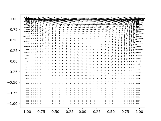
Velocity vectors for Re=100 using Chebyshev

Complete solver

A complete solver can be found in demo NavierStokesDrivenCavity.py.