Demo - Stokes equations

Authors:

Mikael Mortensen (mikaem at math.uio.no)

Date:

January 23, 2019

Summary. The Stokes equations describe the flow of highly viscous fluids. This is a demonstration of how the Python module shenfun can be used to solve Stokes equations using a mixed (coupled) basis in a 3D tensor product domain. We assume homogeneous Dirichlet boundary conditions in one direction and periodicity in the remaining two. The solver described runs with MPI without any further considerations required from the user. The solver assembles a block matrix with sparsity pattern as shown below for the Legendre basis.

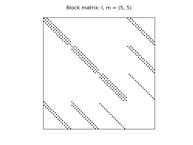
Coupled block matrix for Stokes equations

Stokes’ equations

Stokes’ equations are given in strong form as

\[\begin{split}\begin{align*} \nabla^2 \boldsymbol{u} - \nabla p &= \boldsymbol{f} \quad \text{in } \Omega, \\ \nabla \cdot \boldsymbol{u} &= h \quad \text{in } \Omega, \\ \int_{\Omega} p dx &= 0, \end{align*}\end{split}\]

where \(\boldsymbol{u}\) and \(p\) are, respectively, the fluid velocity vector and pressure, and the domain \(\Omega = [0, 2\pi)^2 \times (-1, 1)\). The flow is assumed periodic in \(x\) and \(y\)-directions, whereas there is a no-slip homogeneous Dirichlet boundary condition on \(\boldsymbol{u}\) on the boundaries of the \(z\)-direction, i.e., \(\boldsymbol{u}(x, y, \pm 1) = (0, 0, 0)\). (Note that we can configure shenfun with non-periodicity in any of the three directions. However, since we are to solve linear algebraic systems in the non-periodic direction, there is a speed benefit from having the nonperiodic direction last. This has to do with Numpy using a C-style row-major storage of arrays by default.) The right hand side vector \(\boldsymbol{f}(\boldsymbol{x})\) is an external applied body force. The right hand side \(h\) is usually zero in the regular Stokes equations. Here we include it because it will be nonzero in the verification, which is using the method of manufactured solutions. Note that the final \(\int_{\Omega} p dx = 0\) is there because there is no Dirichlet boundary condition on the pressure and the system of equations would otherwise be ill conditioned.

To solve Stokes’ equations with the Galerkin method we need basis functions for both velocity and pressure. A Dirichlet basis will be used for velocity, whereas there is no boundary restriction on the pressure basis. For both three-dimensional bases we will use one basis function for the \(x\)-direction, \(\mathcal{X}(x)\), one for the \(y\)-direction, \(\mathcal{Y}(y)\), and one for the \(z\)-direction, \(\mathcal{Z}(z)\). And then we create three-dimensional basis functions like

(1)\[ v(x, y, z) = \mathcal{X}(x) \mathcal{Y}(y) \mathcal{Z} (z).\]

The basis functions \(\mathcal{X}(x)\) and \(\mathcal{Y}(y)\) are chosen as Fourier exponentials, since these functions are periodic:

(2)\[ \mathcal{X}_l(x) = e^{\imath l x}, \forall \, l \in \boldsymbol{l}^{N_0},\]

(3)\[ \mathcal{Y}_m(y) = e^{\imath m y}, \forall \, m \in \boldsymbol{m}^{N_1},\]

where \(\boldsymbol{l}^{N_0} = (-N_0/2, -N_0/2+1, \ldots, N_0/2-1)\) and \(\boldsymbol{m}^{N_1} = (-N_1/2, -N_1/2+1, \ldots, N_1/2-1)\). The size of the discretized problem in real physical space is \(\boldsymbol{N} = (N_0, N_1, N_2)\), i.e., there are \(N_0 \cdot N_1 \cdot N_2\) quadrature points in total.

The basis functions for \(\mathcal{Z}(z)\) remain to be decided. For the velocity we need homogeneous Dirichlet boundary conditions, and for this we use composite Legendre or Chebyshev polynomials

(4)\[ \mathcal{Z}^0_n(z) = \phi_n(z) - \phi_{n+2}(z), \forall \, n \in \boldsymbol{n}^{N_2-2},\]

where \(\phi_n\) is the n’th Legendre or Chebyshev polynomial of the first kind. \(\boldsymbol{n}^{N_2-2} = (0, 1, \ldots, N_2-3)\), and the zero on \(\mathcal{Z}^0\) is there to indicate the zero value on the boundary.

The pressure basis that comes with no restrictions for the boundary is a little trickier. The reason for this has to do with inf-sup stability. The obvious choice of basis is the regular Legendre or Chebyshev basis, which is denoted as

(5)\[ \mathcal{Z}_n(z) = \phi_n(z), \forall \, n \in \boldsymbol{n}^{N_2}.\]

The problem is that for the natural choice of \(n \in (0, 1, \ldots, N_2-1)\) there is a nullspace and one degree of freedom remains unresolved. It turns out that the proper choice for the pressure basis is simply (5) for \(n \in \boldsymbol{n}^{N_2-2}\). (Also remember that we have to fix \(\int_{\Omega} p dx = 0\).)

With given basis functions we obtain the spaces

(6)\[ V^{N_0} = \text{span}\{ \mathcal{X}_l \}_{l\in\boldsymbol{l}^{N_0}},\]

(7)\[ V^{N_1} = \text{span}\{ \mathcal{Y}_m \}_{m\in\boldsymbol{m}^{N_1}},\]

(8)\[ V^{N_2} = \text{span}\{ \mathcal{Z}_n \}_{n\in\boldsymbol{n}^{N_2-2}},\]

(9)\[ V_0^{N_2} = \text{span}\{ \mathcal{Z}^0_n \}_{n\in\boldsymbol{n}^{N_2-2}},\]

and from these we create two different tensor product spaces

(10)\[ W_0^{\boldsymbol{N}}(\boldsymbol{x}) = V^{N_0}(x) \otimes V^{N_1}(y) \otimes V_0^{N_2}(z),\]

(11)\[ W^{\boldsymbol{N}}(\boldsymbol{x}) = V^{N_0}(x) \otimes V^{N_1}(y) \otimes V^{N_2}(z).\]

The velocity vector is using a mixed basis, such that we will look for solutions \(\boldsymbol{u} \in [W_0^{\boldsymbol{N}}]^3 \, (=W_0^{\boldsymbol{N}} \times W_0^{\boldsymbol{N}} \times W_0^{\boldsymbol{N}})\), whereas we look for the pressure \(p \in W^{\boldsymbol{N}}\). We now formulate a variational problem using the Galerkin method: Find \(\boldsymbol{u} \in [W_0^{\boldsymbol{N}}]^3\) and \(p \in W^{\boldsymbol{N}}\) such that

(12)\[ \int_{\Omega} (\nabla^2 \boldsymbol{u} - \nabla p ) \cdot \overline{\boldsymbol{v}} \, dx_w = \int_{\Omega} \boldsymbol{f} \cdot \overline{\boldsymbol{v}}\, dx_w \quad\forall \boldsymbol{v} \, \in \, [W_0^{\boldsymbol{N}}]^3,\]

(13)\[ \int_{\Omega} \nabla \cdot \boldsymbol{u} \, \overline{q} \, dx_w = \int_{\Omega} h \overline{q} \, dx_w \quad\forall q \, \in \, W^{\boldsymbol{N}}.\]

Here \(dx_w=w_xdxw_ydyw_zdz\) represents a weighted measure, with weights \(w_x(x), w_y(y), w_z(z)\). Note that it is only Chebyshev polynomials that make use of a non-constant weight \(w_x=1/\sqrt{1-x^2}\). The Fourier weights are \(w_y=w_z=1/(2\pi)\) and the Legendre weight is \(w_x=1\). The overline in \(\boldsymbol{\overline{v}}\) and \(\overline{q}\) represents a complex conjugate, which is needed here because the Fourier exponentials are complex functions.

Mixed variational form

Since we are to solve for \(\boldsymbol{u}\) and \(p\) at the same time, we formulate a mixed (coupled) problem: find \((\boldsymbol{u}, p) \in [W_0^{\boldsymbol{N}}]^3 \times W^{\boldsymbol{N}}\) such that

(14)\[ a((\boldsymbol{u}, p), (\boldsymbol{v}, q)) = L((\boldsymbol{v}, q)) \quad \forall (\boldsymbol{v}, q) \in [W_0^{\boldsymbol{N}}]^3 \times W^{\boldsymbol{N}},\]

where bilinear (\(a\)) and linear (\(L\)) forms are given as

(15)\[ a((\boldsymbol{u}, p), (\boldsymbol{v}, q)) = \int_{\Omega} (\nabla^2 \boldsymbol{u} - \nabla p) \cdot \overline{\boldsymbol{v}} \, dx_w + \int_{\Omega} \nabla \cdot \boldsymbol{u} \, \overline{q} \, dx_w,\]

(16)\[ L((\boldsymbol{v}, q)) = \int_{\Omega} \boldsymbol{f} \cdot \overline{\boldsymbol{v}}\, dx_w + \int_{\Omega} h \overline{q} \, dx_w.\]

Note that the bilinear form will assemble to block matrices, whereas the right hand side linear form will assemble to block vectors.

Implementation

Preamble

We will solve the Stokes equations using the shenfun Python module. The first thing needed is then to import some of this module’s functionality plus some other helper modules, like Numpy and Sympy:

import os
import sys
import numpy as np
from sympy import symbols, sin, cos
from shenfun import *

We use Sympy for the manufactured solution and Numpy for testing.

Manufactured solution

The exact solutions \(\boldsymbol{u}_e(\boldsymbol{x})\) and \(p(\boldsymbol{x})\) are chosen to satisfy boundary conditions, and the right hand sides \(\boldsymbol{f}(\boldsymbol{x})\) and \(h(\boldsymbol{x})\) are then computed exactly using Sympy. These exact right hand sides will then be used to compute a numerical solution that can be verified against the manufactured solution. The chosen solution with computed right hand sides are:

x, y, z = symbols('x,y,z')
uex = sin(2*y)*(1-z**2)
uey = sin(2*x)*(1-z**2)
uez = sin(2*z)*(1-z**2)
pe = -0.1*sin(2*x)*cos(4*y)
fx = uex.diff(x, 2) + uex.diff(y, 2) + uex.diff(z, 2) - pe.diff(x, 1)
fy = uey.diff(x, 2) + uey.diff(y, 2) + uey.diff(z, 2) - pe.diff(y, 1)
fz = uez.diff(x, 2) + uez.diff(y, 2) + uez.diff(z, 2) - pe.diff(z, 1)
h = uex.diff(x, 1) + uey.diff(y, 1) + uez.diff(z, 1)

Tensor product spaces

One-dimensional spaces are created using the FunctionSpace() function. A choice of polynomials between Legendre or Chebyshev can be made, and the size of the domain is given

N = (20, 20, 20)
family = 'Legendre'
K0 = FunctionSpace(N[0], 'Fourier', dtype='D', domain=(0, 2*np.pi))
K1 = FunctionSpace(N[1], 'Fourier', dtype='d', domain=(0, 2*np.pi))
SD = FunctionSpace(N[2], family, bc=(0, 0))
ST = FunctionSpace(N[2], family)

Next the one-dimensional spaces are used to create two tensor product spaces Q = \(W^{\boldsymbol{N}}\) and TD = \(W_0^{\boldsymbol{N}}\), one vector V = \([W_0^{\boldsymbol{N}}]^3\) and one mixed space VQ = V \(\times\) Q.

TD = TensorProductSpace(comm, (K0, K1, SD), axes=(2, 0, 1))
Q = TensorProductSpace(comm, (K0, K1, ST), axes=(2, 0, 1))
V = VectorSpace(TD)
VQ = CompositeSpace([V, Q])

Note that we choose to transform axes in the order \(1, 0, 2\). This is to ensure that the fully transformed arrays are aligned in the non-periodic direction 2. And we need the arrays aligned in this direction, because this is the only direction where there are tensor product matrices that are non-diagonal. All Fourier matrices are, naturally, diagonal.

Test- and trialfunctions are created much like in a regular, non-mixed, formulation. However, one has to create one test- and trialfunction for the mixed space, and then split them up afterwards

up = TrialFunction(VQ)
vq = TestFunction(VQ)
u, p = up
v, q = vq

With the basisfunctions in place we may assemble the different blocks of the final coefficient matrix. Since Legendre is using a constant weight function, the equations may also be integrated by parts to obtain a symmetric system:

if family.lower() == 'chebyshev':
    A = inner(v, div(grad(u)))
    G = inner(v, -grad(p))
else:
    A = inner(grad(v), -grad(u))
    G = inner(div(v), p)
D = inner(q, div(u))

The assembled subsystems A, G and D are lists containg the different blocks of the complete, coupled matrix. A actually contains 6 tensor product matrices of type TPMatrix. The first two matrices are for vector component zero of the test function v[0] and trial function u[0], the matrices 2 and 3 are for components 1 and the last two are for components 2. The first two matrices are as such for

A[0:2] = inner(v[0], div(grad(u[0])))

Breaking it down this inner product is mathematically

(17)\[ \int_{\Omega} \boldsymbol{\overline{v}}[0] \left(\frac{\partial^2 \boldsymbol{u}[0]}{\partial x^2} + \frac{\partial^2 \boldsymbol{u}[0]}{\partial y^2} + \frac{\partial^2 \boldsymbol{u}[0]}{\partial z^2}\right) w_x dx w_y dy w_z dz.\]

If we now use test function \(\boldsymbol{v}[0]\)

(18)\[ \boldsymbol{v}[0]_{lmn} = \mathcal{X}_l \mathcal{Y}_m \mathcal{Z}_n,\]

and trialfunction

(19)\[ \boldsymbol{u}[0]_{pqr} = \sum_{p} \sum_{q} \sum_{r} \hat{\boldsymbol{u}}[0]_{pqr} \mathcal{X}_p \mathcal{Y}_q \mathcal{Z}_r,\]

where \(\hat{\boldsymbol{u}}\) are the unknown degrees of freedom, and then insert these functions into (17), then we obtain after performing some exact evaluations over the periodic directions

(20)\[ \Big( \underbrace{-\left(l^2 \delta_{lp} + m^2 \delta_{mq} \right) \int_{-1}^{1} \mathcal{Z}_r(z) \mathcal{Z}_n(z) w_z dz}_{A[0]} + \underbrace{\delta_{lp} \delta_{mq} \int_{-1}^{1} \frac{\partial^2 \mathcal{Z}_r(z)}{\partial z^2} \mathcal{Z}_n(z) w_z dz}_{A[1]} \Big) \hat{\boldsymbol{u}}[0]_{pqr}.\]

Similarly for components 1 and 2 of the test and trial vectors, leading to 6 tensor product matrices in total for A. Similarly, we get three components of G and three of D.

Eliminating the Fourier diagonal matrices, we are left with block matrices like

\[\begin{split}H(l, m) = \begin{bmatrix} A[0]+A[1] & 0 & 0 & G[0] \\ 0 & A[2]+A[3] & 0 & G[1] \\ 0 & 0 & A[4]+A[5] & G[2] \\ D[0] & D[1] & D[2] & 0 \end{bmatrix}\end{split}\]

Note that there will be one large block matrix \(H(l, m)\) for each Fourier wavenumber combination \((l, m)\). To solve the problem in the end we will need to loop over these wavenumbers and solve the assembled linear systems one by one. An example of the block matrix, for \(l=m=5\) and \(\boldsymbol{N}=(20, 20, 20)\) is given in Fig. Coupled block matrix for Stokes equations.

In the end we create a block matrix through

M = BlockMatrix(A+G+D)

The right hand side can easily be assembled since we have already defined the functions \(\boldsymbol{f}\) and \(h\), see Sec. Manufactured solution

# Get mesh (quadrature points)
X = TD.local_mesh(True)

# Get f and h on quad points
fh = Array(VQ, buffer=(fx, fy, fz, h))
f_, h_ = fh

# Compute inner products
fh_hat = Function(VQ)
f_hat, h_hat = fh_hat
f_hat = inner(v, f_, output_array=f_hat)
h_hat = inner(q, h_, output_array=h_hat)

In the end all that is left is to solve and compare with the exact solution.

# Solve problem
up_hat = M.solve(fh_hat, constraints=((3, 0, 0), (3, N[2]-1, 0)))
up = up_hat.backward()
u_, p_ = up

# Exact solution
ux, uy, uz = Array(V, buffer=(uex, uey, uez))
pe = Array(Q, buffer=pe)

error = [comm.reduce(np.linalg.norm(ux-u_[0])),
         comm.reduce(np.linalg.norm(uy-u_[1])),
         comm.reduce(np.linalg.norm(uz-u_[2])),
         comm.reduce(np.linalg.norm(pe-p_))]
print(error)

Note that solve has a keyword argument constraints=((3, 0, 0), (3, N[2]-1), 0) that takes care of the restriction \(\int_{\Omega} p \omega dx = 0\) by indenting the rows in M corresponding to the first and last degree of freedom for the pressure. The value \((3, 0, 0)\) indicates that pressure is in block 3 of the block vector solution (the velocity vector holds positions 0, 1 and 2), whereas the two zeros ensures that the first dof (dof 0) should obtain value 0. The constraint on the highest wavenumber (3, N[2]-1, 0) is required to get a non-singular matrix.

Complete solver

A complete solver can be found in demo Stokes3D.py.