Demo - Working with Functions

Mikael Mortensen (email: mikaem@math.uio.no), Department of Mathematics, University of Oslo.

Date: August 7, 2020

Summary. This is a demonstration of how the Python module shenfun can be used to work with global spectral functions in one and several dimensions.

Construction

A global spectral function \(u(x)\) can be represented on the real line as

\[u(x) = \sum_{k=0}^{N-1} \hat{u}_k \psi_k(x), \quad x \in \Omega = [a, b],\]

where the domain \(\Omega\) has to be defined such that \(b > a\). The array \(\{\hat{u}_k\}_{k=0}^{N-1}\) contains the expansion coefficient for the series, often referred to as the degrees of freedom. There is one degree of freedom per basis function and \(\psi_k(x)\) is the \(k\)’th basis function. We can use any number of basis functions, and the span of the chosen basis is then a function space. Also part of the function space is the domain, which is specified when a function space is created. To create a function space \(T=\text{span}\{T_k\}_{k=0}^{N-1}\) for the first N Chebyshev polynomials of the first kind on the default domain \([-1, 1]\), do

from shenfun import *
N = 8
T = FunctionSpace(N, 'Chebyshev', domain=(-1, 1))

The function \(u(x)\) can now be created with all N coefficients equal to zero as

u = Function(T)

When using Chebyshev polynomials the computational domain is always \([-1, 1]\). However, we can still use a different physical domain, like

T = FunctionSpace(N, 'Chebyshev', domain=(0, 1))

and under the hood shenfun will then map this domain to the reference domain through

\[u(x) = \sum_{k=0}^{N-1} \hat{u}_k \psi_k(2(x-0.5))\]

Approximating analytical functions

The u function above was created with only zero valued coefficients, which is the default. Alternatively, a Function may be initialized using a constant value

T = FunctionSpace(N, 'Chebyshev', domain=(-1, 1))
u = Function(T, val=1)

but that is not very useful. A third method to initialize a Function is to interpolate using an analytical Sympy function.

import sympy as sp
x = sp.Symbol('x', real=True)
u = Function(T, buffer=4*x**3-3*x)
print(u)

[-6.93889390e-17 -5.47405982e-17 -1.82237827e-18  1.00000000e+00
  1.96261557e-17 -3.33066907e-16  1.49457239e-16 -2.93881977e-16]

Here the analytical Sympy function will first be evaluated on the entire quadrature mesh of the T function space, and then forward transformed to get the coefficients. This corresponds to a finite-dimensional projection to T. The projection is

Find \(u_h \in T\), such that

\[(u_h - u, v)^{N}_w = 0 \quad \forall v \in T, \label{eq:proj1} \tag{1}\]

where \(v\) is a test function and \(u_h=\sum_{k=0}^{N-1} \hat{u}_k T_k\) is a trial function. The notation \((\cdot, \cdot)^N_w\) represents a discrete version of the weighted inner product \((u, v)_w\) defined as

\[(u, v)_{\omega} = \int_{\Omega} u \overline{v} \omega d\Omega,\]

where \(\omega(x)\) is a weight functions and \(\overline{v}\) is the complex conjugate of \(v\). If \(v\) is a real function, then \(\overline{v}=v\). With quadrature we approximate the integral such that

\[(u, v)_{\omega} \approx (u, v)^N_{\omega} = \sum_{j\in\mathcal{I}^N} u(x_j) v(x_j) w_j.\]

where the index set \(\mathcal{I}^N = \{0, 1, \ldots, N-1\}\) and \(\{x_j\}_{j\in \mathcal{I}^N}\) and \(\{w_j\}_{j\in \mathcal{I}^N}\) are the quadrature points and weights.

A linear system of equations arise when inserting for the chosen basis functions in Eq. (1). We get

\[\sum_{k\in \mathcal{I}^N} \left( T_k, T_i\right)^N_{\omega} \hat{u}_k = \left(u, T_i\right)^N_{\omega}\, \forall \, i \in \mathcal{I}^N,\]

In matrix notation the solution becomes

\[\boldsymbol{\hat{u}} = A^{-1} \boldsymbol{\tilde{u}},\]

where we use two column vectors \(\boldsymbol{\hat{u}}=(\hat{u}_i)^T_{i\in \mathcal{I}^N}\), \(\boldsymbol{\tilde{u}}=\left(\tilde{u}_i\right)^T_{i \in \mathcal{I}^N}\), \(\tilde{u}_i = (u, T_i)^N_{\omega}\) and the matrix \(A=(a_{ik}) \in \mathbb{R}^{N \times N}\), that is diagonal with \(a_{ik}=\left( T_k, T_i\right)^N_{\omega}\). For the default Gauss-Chebyshev quadrature this matrix is \(a_{ik} = c_i \pi/2 \delta_{ik}\), where \(c_0=2\) and \(c_i=1\) for \(i>0\).

Adaptive function size

The number of basis functions can also be left open during creation of the function space, through

T = FunctionSpace(0, 'Chebyshev', domain=(-1, 1))

This is useful if you want to approximate a function and are uncertain how many basis functions that are required. For example, you may want to approximate the function \(\cos(20 x)\). You can then find the required Function using

u = Function(T, buffer=sp.cos(20*x))
print(len(u))

37

We see that \(N=45\) is required to resolve this function. This agrees well with what is reported also by Chebfun. Note that in this process a new FunctionSpace() has been created under the hood. The function space of u can be extracted using

Tu = u.function_space()
print(Tu.N)

37

To further show that shenfun is compatible with Chebfun we can also approximate the Bessel function

T1 = FunctionSpace(0, 'Chebyshev', domain=(0, 100))
u = Function(T1, buffer=sp.besselj(0, x))
print(len(u))

83

which gives 83 basis functions, in close agreement with Chebfun (89). The difference lies only in the cut-off criteria. We cut frequencies with a relative tolerance of 1e-12 by default, but if we make this criteria a little bit stronger, then we will also arrive at a slightly higher number:

u = Function(T1, buffer=sp.besselj(0, x), reltol=1e-14)
print(len(u))

87

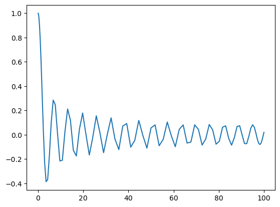
Plotting the function on its quadrature points looks a bit ragged, though:

%matplotlib inline

import matplotlib.pyplot as plt
Tu = u.function_space()
plt.plot(Tu.mesh(), u.backward());

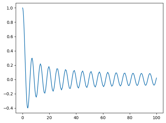
To improve the quality of this plot we can instead evaluate the function on more points

xj = np.linspace(0, 100, 1000)
plt.plot(xj, u(xj));

Alternatively, we can refine the function, which simply pads zeros to \(\hat{u}\)

up = u.refine(200)
Tp = up.function_space()
plt.plot(Tp.mesh(), up.backward());

The padded expansion coefficients are now given as

print(up)

[ 6.43655435e-02 -1.37262942e-01  1.26593632e-01 -1.31630372e-01
  1.19810309e-01 -1.19499576e-01  1.07387826e-01 -9.95196201e-02
  8.81197795e-02 -7.07299943e-02  6.13974837e-02 -3.40222966e-02
  2.84578300e-02  6.05886310e-03 -6.23468323e-03  4.01956708e-02
 -3.44202241e-02  5.58353154e-02 -4.58848577e-02  4.33923041e-02
 -3.39778387e-02  6.26445963e-03 -3.37831264e-03 -3.27304442e-02
  2.63630973e-02 -4.12313235e-02  3.07429560e-02 -7.73458857e-03
  4.10441868e-03  3.29922472e-02 -2.47812478e-02  2.71654360e-02
 -1.81421444e-02 -2.02112290e-02  1.53660102e-02 -3.02943723e-02
  1.97324599e-02  1.94051084e-02 -1.41460820e-02  2.47321146e-02
 -1.49668436e-02 -3.02763148e-02  1.98156190e-02 -2.08517347e-03
 -6.91643640e-05  3.13799203e-02 -1.81924272e-02 -3.77110141e-02
  2.23051599e-02  2.82766986e-02 -1.67226896e-02 -1.59965877e-02
  9.40673776e-03  7.34392211e-03 -4.28398348e-03 -2.84497604e-03
  1.64428109e-03  9.53197714e-04 -5.45450869e-04 -2.80998822e-04
  1.59136941e-04  7.38240716e-05 -4.13664358e-05 -1.74579288e-05
  9.67744748e-06  3.74610168e-06 -2.05413769e-06 -7.34256601e-07
  3.98257402e-07  1.32202237e-07 -7.09282453e-08 -2.19709845e-08
  1.16601214e-08  3.38459230e-09 -1.77684428e-09 -4.85085285e-10
  2.51925667e-10  6.48958256e-11 -3.33432158e-11 -8.12799381e-12
  4.13195149e-12  9.55498771e-13 -4.80687010e-13 -1.05592419e-13
  5.24752655e-14  1.10454430e-14 -6.02774535e-15  0.00000000e+00
  0.00000000e+00  0.00000000e+00  0.00000000e+00  0.00000000e+00
  0.00000000e+00  0.00000000e+00  0.00000000e+00  0.00000000e+00
  0.00000000e+00  0.00000000e+00  0.00000000e+00  0.00000000e+00
  0.00000000e+00  0.00000000e+00  0.00000000e+00  0.00000000e+00
  0.00000000e+00  0.00000000e+00  0.00000000e+00  0.00000000e+00
  0.00000000e+00  0.00000000e+00  0.00000000e+00  0.00000000e+00
  0.00000000e+00  0.00000000e+00  0.00000000e+00  0.00000000e+00
  0.00000000e+00  0.00000000e+00  0.00000000e+00  0.00000000e+00
  0.00000000e+00  0.00000000e+00  0.00000000e+00  0.00000000e+00
  0.00000000e+00  0.00000000e+00  0.00000000e+00  0.00000000e+00
  0.00000000e+00  0.00000000e+00  0.00000000e+00  0.00000000e+00
  0.00000000e+00  0.00000000e+00  0.00000000e+00  0.00000000e+00
  0.00000000e+00  0.00000000e+00  0.00000000e+00  0.00000000e+00
  0.00000000e+00  0.00000000e+00  0.00000000e+00  0.00000000e+00
  0.00000000e+00  0.00000000e+00  0.00000000e+00  0.00000000e+00
  0.00000000e+00  0.00000000e+00  0.00000000e+00  0.00000000e+00
  0.00000000e+00  0.00000000e+00  0.00000000e+00  0.00000000e+00
  0.00000000e+00  0.00000000e+00  0.00000000e+00  0.00000000e+00
  0.00000000e+00  0.00000000e+00  0.00000000e+00  0.00000000e+00
  0.00000000e+00  0.00000000e+00  0.00000000e+00  0.00000000e+00
  0.00000000e+00  0.00000000e+00  0.00000000e+00  0.00000000e+00
  0.00000000e+00  0.00000000e+00  0.00000000e+00  0.00000000e+00
  0.00000000e+00  0.00000000e+00  0.00000000e+00  0.00000000e+00
  0.00000000e+00  0.00000000e+00  0.00000000e+00  0.00000000e+00
  0.00000000e+00  0.00000000e+00  0.00000000e+00  0.00000000e+00
  0.00000000e+00  0.00000000e+00  0.00000000e+00  0.00000000e+00
  0.00000000e+00  0.00000000e+00  0.00000000e+00  0.00000000e+00
  0.00000000e+00  0.00000000e+00  0.00000000e+00  0.00000000e+00]

More features

Since we have used a regular Chebyshev basis above, there are many more features that could be explored simply by going through Numpy’s Chebyshev module. For example, we can create a Chebyshev series like

import numpy.polynomial.chebyshev as cheb
c = cheb.Chebyshev(u, domain=(0, 100))

The Chebyshev series in Numpy has a wide range of possibilities, see here. However, we may also work directly with the Chebyshev coefficients already in u. To find the roots of the polynomial that approximates the Bessel function on domain \([0, 100]\), we can do

z = Tu.map_true_domain(cheb.chebroots(u))

Note that the roots are found on the reference domain \([-1, 1]\) and as such we need to move the result to the physical domain using map_true_domain. The resulting roots z are both real and imaginary, so to extract the real roots we need to filter a little bit

z2 = z[np.where((z.imag == 0)*(z.real > 0)*(z.real < 100))].real
print(z2[:5])

[ 2.40482556  5.52007811  8.65372791 11.79153444 14.93091771]

Here np.where returns the indices where the condition is true. The condition is that the imaginary part is zero, whereas the real part is within the true domain \([0, 100]\).

Notice.

Using directly cheb.chebroots(c) does not seem to work (even though the series has been generated with the non-standard domain) because Numpy only looks for roots in the reference domain \([-1, 1]\).

We could also use a function space with boundary conditions built in, like

Td = FunctionSpace(0, 'C', bc=(sp.besselj(0, 0), sp.besselj(0, 100)), domain=(0, 100))
ud = Function(Td, buffer=sp.besselj(0, x))
print(len(ud))

82

As we can see this leads to a function space of dimension very similar to the orthogonal space.

The major advantages of working with a space with boundary conditions built in only comes to life when solving differential equations. As long as we are only interested in approximating functions, we are better off sticking to the orthogonal spaces. This goes for Legendre as well as Chebyshev.

Multidimensional functions

Multidimensional tensor product spaces are created by taking the tensor products of one-dimensional function spaces. For example

C0 = FunctionSpace(20, 'C')
C1 = FunctionSpace(20, 'C')
T = TensorProductSpace(comm, (C0, C1))
u = Function(T)

Here \(\text{T} = \text{C0} \otimes \text{C1}\), the basis function is \(T_i(x) T_j(y)\) and the Function u is

\[u(x, y) = \sum_{i=0}^{N-1} \sum_{j=0}^{N-1} \hat{u}_{ij} T_i(x) T_j(y).\]

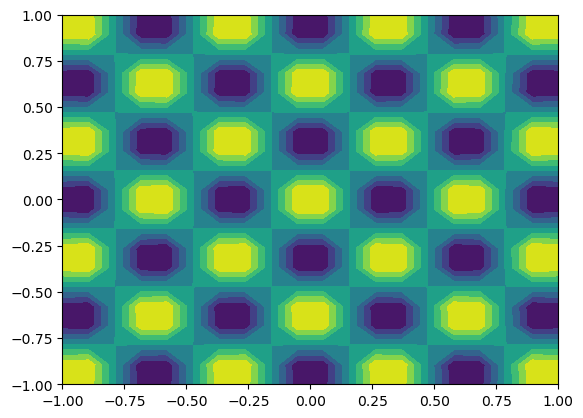
The multidimensional Functions work more or less exactly like for the 1D case. We can here interpolate 2D Sympy functions

y = sp.Symbol('y', real=True)
u = Function(T, buffer=sp.cos(10*x)*sp.cos(10*y))
X = T.local_mesh(True)
plt.contourf(X[0], X[1], u.backward());

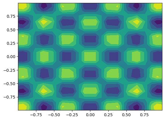
Like for 1D the coefficients are computed through projection, where the exact function is evaluated on all quadrature points in the mesh.

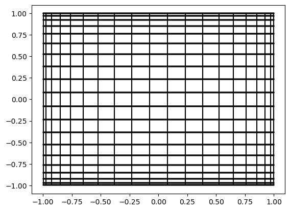
The Cartesian mesh represents the quadrature points of the two function spaces, and can be visualized as follows

X = T.mesh()
for xj in X[0]:
    for yj in X[1]:
        plt.plot((xj, xj), (X[1][0, 0], X[1][0, -1]), 'k')
        plt.plot((X[0][0], X[0][-1]), (yj, yj), 'k')

We may alternatively plot on a uniform mesh

X = T.local_mesh(bcast=True, kind='uniform')
plt.contourf(X[0], X[1], u.backward(mesh='uniform'));

Curvilinear coordinates

With shenfun it is possible to use curvilinear coordinates, and not necessarily with orthogonal basis vectors. With curvilinear coordinates the computational coordinates are always straight lines, rectangles and cubes. But the physical coordinates can be very complex.

Consider the unit disc with polar coordinates. Here the position vector \(\mathbf{r}\) is given by

\[\mathbf{r} = r\cos \theta \mathbf{i} + r\sin \theta \mathbf{j}.\]

The physical domain is \(\Omega = \{(x, y): x^2 + y^2 < 1\}\), whereas the computational domain is the Cartesian product \(D = [0, 1] \times [0, 2 \pi] = \{(r, \theta) | r \in [0, 1] \text{ and } \theta \in [0, 2 \pi]\}\).

We create this domain in shenfun through

r, theta = psi = sp.symbols('x,y', real=True, positive=True)
rv = (r*sp.cos(theta), r*sp.sin(theta))
B0 = FunctionSpace(20, 'C', domain=(0, 1))
F0 = FunctionSpace(20, 'F')
T = TensorProductSpace(comm, (B0, F0), coordinates=(psi, rv))

Note that we are using a Fourier space for the azimuthal direction, since the solution here needs to be periodic. We can now create functions on the space using an analytical function in computational coordinates

u = Function(T, buffer=(1-r)*r*sp.sin(sp.cos(theta)))

However, when this is plotted it may not be what you expect

X = T.local_mesh(True)
plt.contourf(X[0], X[1], u.backward(), 100);

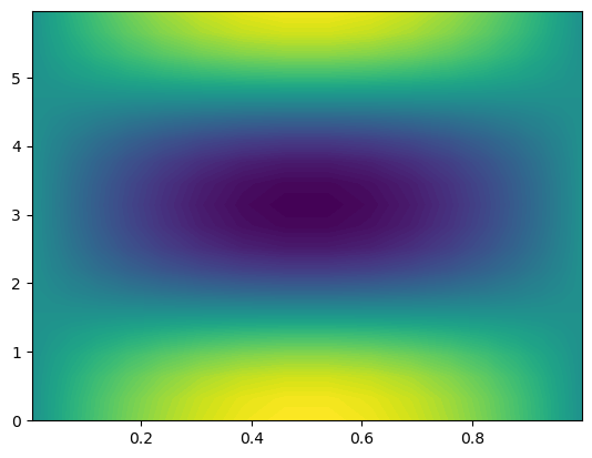
We see that the function has been plotted in computational coordinates, and not on the disc, as you probably expected. To plot on the disc we need the physical mesh, and not the computational

X = T.local_cartesian_mesh()
plt.contourf(X[0], X[1], u.backward(), 100);

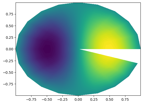
Notice.

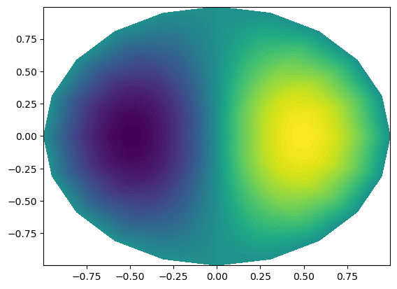
The periodic plot does not wrap all around the circle. This is not wrong, we have simply not used the same point twice, but it does not look very good. To overcome this problem we can wrap the grid all the way around and re-plot.

up = u.backward()
xp, yp, up = wrap_periodic([X[0], X[1], up], axes=[1])
plt.contourf(xp, yp, up, 100);

Adaptive functions in multiple dimensions

If you want to find a good resolution for a function in multiple dimensions, the procedure is exactly like in 1D. First create function spaces with 0 quadrature points, and then call Function

B0 = FunctionSpace(0, 'C', domain=(0, 1))
F0 = FunctionSpace(0, 'F')
T = TensorProductSpace(comm, (B0, F0), coordinates=(psi, rv))
u = Function(T, buffer=((1-r)*r)**2*sp.sin(sp.cos(theta)))
print(u.shape)

(5, 12)

The algorithm used to find the approximation in multiple dimensions simply treat the problem one direction at the time. So in this case we would first find a space in the first direction by using a function ~ ((1-r)*r)**2, and then along the second using a function ~ sp.sin(sp.cos(theta)).