Demo - Rayleigh Benard
Mikael Mortensen (email: mikaem@math.uio.no), Department of Mathematics, University of Oslo.
Date: November 21, 2019
Summary. Rayleigh-Benard convection arise due to temperature gradients in a fluid. The governing equations are Navier-Stokes coupled (through buoyancy) with an additional temperature equation derived from the first law of thermodynamics, using a linear correlation between density and temperature.
This is a demonstration of how the Python module shenfun can be used to solve for these Rayleigh-Benard cells in a 2D channel with two walls of different temperature in one direction, and periodicity in the other direction. The solver described runs with MPI without any further considerations required from the user. Note that there is also a more physically realistic 3D solver. The solver described in this demo has been implemented in a class in the RayleighBenard2D.py module in the demo folder of shenfun. Below is an example solution, which has been run at a very high Rayleigh number (Ra).
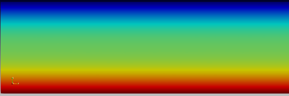
Figure 1: Temperature fluctuations in the Rayleigh Benard flow. The top and bottom walls are kept at different temperatures and this sets up the Rayleigh-Benard convection. The simulation is run at Ra =1,000,000, Pr =0.7 with 256 and 512 quadrature points in x and y-directions, respectively.
The Rayleigh Bénard equations
The governing equations solved in domain \(\Omega=(-1, 1)\times [0, 2\pi)\) are
where \(\boldsymbol{u}(x, y, t) (= u\boldsymbol{i} + v\boldsymbol{j})\) is the velocity vector, \(p(x, y, t)\) is pressure, \(T(x, y, t)\) is the temperature, and \(\boldsymbol{i}\) and \(\boldsymbol{j}\) are the unity vectors for the \(x\) and \(y\)-directions, respectively.
The equations are complemented with boundary conditions \(\boldsymbol{u}(\pm 1, y, t) = (0, 0), \boldsymbol{u}(x, 2 \pi, t) = \boldsymbol{u}(x, 0, t), T(-1, y, t) = 1, T(1, y, t) = 0, T(x, 2 \pi, t) = T(x, 0, t)\). Note that these equations have been non-dimensionalized according to [pandey18], using dimensionless Rayleigh number \(Ra=g \alpha \Delta T h^3/(\nu \kappa)\) and Prandtl number \(Pr=\nu/\kappa\). Here \(g \boldsymbol{i}\) is the vector accelleration of gravity, \(\Delta T\) is the temperature difference between the top and bottom walls, \(h\) is the hight of the channel in \(x\)-direction, \(\nu\) is the dynamic viscosity coefficient, \(\kappa\) is the heat transfer coefficient and \(\alpha\) is the thermal expansion coefficient. Note that the governing equations have been non-dimensionalized using the free-fall velocityscale \(U=\sqrt{g \alpha \Delta T h}\). See [pandey18] for more details.
The governing equations contain a non-trivial coupling between velocity, pressure and temperature. This coupling can be simplified by eliminating the pressure from the equation for the wall-normal velocity component \(u\). We accomplish this by taking the Laplace of the momentum equation in wall normal direction, using the pressure from the divergence of the momentum equation \(\nabla^2 p = -\nabla \cdot \boldsymbol{H}+\partial T/\partial x\), where \(\boldsymbol{H} = (H_x, H_y) = (\boldsymbol{u} \cdot \nabla) \boldsymbol{u}\)
This equation is solved with \(u(\pm 1,y,t) = \partial u/\partial x(\pm 1,y,t) = 0\), where the latter follows from the divergence constraint. In summary, we now seem to have the following equations to solve:
However, we note that Eqs. (5) and (7) and (8) do not depend on pressure, and, apparently, on each time step we can solve (5) for \(u\), then (8) for \(v\) and finally (7) for \(T\). So what do we need (6) for? It appears to have become redundant from the elimination of the pressure from Eq. (5). It turns out that this is actually almost completely true, but (5), (7) and (8) can only provide closure for all but one of the Fourier coefficients. To see this it is necessary to introduce some discretization and basis functions that will be used to solve the problem. To this end we use \(P_N\), which is the set of all real polynomials of degree less than or equal to N and introduce the following finite-dimensional approximation spaces
Here \(\text{dim}(V_N^B) = N-4, \text{dim}(V_N^D) = \text{dim}(V_N^W) = \text{dim}(V_N^T) = N-2\) and \(\text{dim}(V_M^F)=M\). We note that \(V_N^B, V_N^D, V_N^W\) and \(V_N^T\) can be used to approximate \(u, v, T\) and \(p\), respectively, in the \(x\)-direction. Also note that for \(V_M^F\) it is assumed that \(M\) is an even number.
We can now choose basis functions for the spaces, using Shen’s composite bases for either Legendre or Chebyshev polynomials. For the Fourier space the basis functions are already given. We leave the actual choice of basis as an implementation option for later. For now we use \(\phi^B(x), \phi^D(x), \phi^W\) and \(\phi^T(x)\) as common notation for basis functions in spaces \(V_N^B, V_N^D, V_N^W\) and \(V_N^T\), respectively.
To get the required approximation spaces for the entire domain we use tensor products of the one-dimensional spaces in (9)-(13)
Space \(W_{BF}\) has 2D tensor product basis functions \(\phi_k^B(x) \exp (\imath l y)\) and similar for the others. All in all we get the following approximations for the unknowns
where \(\boldsymbol{k}_{x} = \{0, 1, \ldots \text{dim}(V_N^x)-1\}, \, \text{for} \, x\in(B, D, W, T)\) and \(\boldsymbol{l} = \{-M/2, -M/2+1, \ldots, M/2-1\}\). Note that since the problem is defined in real space we will have Hermitian symmetry. This means that \(\hat{u}_{k, l} = \overline{\hat{u}}_{k, -l}\), with an overbar being a complex conjugate, and similar for \(\hat{v}_{kl}, \hat{p}_{kl}\) and \(\hat{T}_{kl}\). For this reason we can get away with solving for only the positive \(l\)’s, as long as we remember that the sum in the end goes over both positive and negative \(l's\). This is actually automatically taken care of by the FFT provider and is not much of an additional complexity in the implementation. So from now on \(\boldsymbol{l} = \{0, 1, \ldots, M/2\}\).
We can now take a look at why Eq. (6) is needed. If we first solve (5) for \(\hat{u}_{kl}(t), (k, l) \in \boldsymbol{k}_B \times \boldsymbol{l}\), then we can use (8) to solve for \(\hat{v}_{kl}(t)\). But here there is a problem. We can see this by creating the variational form required to solve (8) by the spectral Galerkin method. To this end make \(v=v_N\) in (8) a trial function, use \(u=u_N\) a known function and take the weighted inner product over the domain using test function \(q \in W_{DF}\)
Here we are using the inner product notation
where the exact form of the weighted scalar product depends on the chosen basis; Legendre has \(dx_w=dx\), Chebyshev \(dx_w = dx/\sqrt{1-x^2}\) and Fourier \(dy_w=dy/2/\pi\). The bases also have associated quadrature weights \(\{w_i \}_{i=0}^{N-1}\) and \(\{w_j\}_{j=0}^{M-1}\) that are used to approximate the integrals.
Inserting now for the known \(u_N\), the unknown \(v_N\), and \(q=\phi_m^D(x) \exp(\imath n y)\) the continuity equation becomes
The \(x\) and \(y\) domains are separable, so we can rewrite as
Now perform some exact manipulations in the Fourier direction and introduce the 1D inner product notation for the \(x\)-direction
By also simplifying the notation using summation of repeated indices, we get the following equation
Now \(l\) must equal \(n\) and we can simplify some more
We see that this equation can be solved for \(\hat{v}_{kl} \text{ for } (k, l) \in \boldsymbol{k}_D \times [1, 2, \ldots, M/2]\), but try with \(l=0\) and you hit division by zero, which obviously is not allowed. And this is the reason why Eq. (6) is still needed, to solve for \(\hat{v}_{k,0}\)! Fortunately, since \(\exp(\imath 0 y) = 1\), the pressure derivative \(\frac{\partial p}{\partial y} = 0\), and as such the pressure is still not required. When used only for Fourier coefficient 0, Eq. (6) becomes
There is still one more revelation to be made from Eq. (26). When \(l=0\) we get
which is trivially satisfied if \(\hat{u}_{k,0}=0\) for \(k\in\boldsymbol{k}_B\). Bottom line is that we only need to solve Eq. (5) for \(l \in \boldsymbol{l}/\{0\}\), whereas we can use directly \(\hat{u}_{k,0}=0 \text{ for } k \in \boldsymbol{k}_B\).
To sum up, with the solution known at \(t = t - \Delta t\), we solve
Equation |
For unknown |
With indices |
|---|---|---|
(5) |
\(\hat{u}_{kl}(t)\) |
\((k, l) \in \boldsymbol{k}_B \times \boldsymbol{l}\) |
(8) |
\(\hat{v}_{kl}(t)\) |
\((k, l) \in \boldsymbol{k}_D \times \boldsymbol{l}/\{0\}\) |
(27) |
\(\hat{v}_{kl}(t)\) |
\((k, l) \in \boldsymbol{k}_D \times \{0\}\) |
(7) |
\(\hat{T}_{kl}(t)\) |
\((k, l) \in \boldsymbol{k}_T \times \boldsymbol{l}\) |
Temporal discretization
The governing equations are integrated in time using any one of the time steppers available in shenfun. There are several possible IMEX Runge Kutta methods, see integrators.py. The time steppers are used for any generic equation
where \(\mathcal{N}\) and \(\mathcal{L}\) represents the nonlinear and linear contributions, respectively. The timesteppers are provided with \(\psi, \mathcal{L}\) and \(\mathcal{N}\), and possibly some tailored linear algebra solvers, and solvers are then further assembled under the hood.
All the timesteppers split one time step into one or several stages. The classes IMEXRK222, IMEXRK3 and IMEXRK443 have 2, 3 and 4 steps, respectively, and the cost is proportional.
Implementation
To get started we need instances of the approximation spaces discussed in Eqs. (9) - (17). When the spaces are created we also need to specify the family and the dimension of each space. Here we simply choose Chebyshev and Fourier with 100 and 256 quadrature points in \(x\) and \(y\)-directions, respectively. We could replace ‘Chebyshev’ by ‘Legendre’, but the former is known to be faster due to the existence of fast transforms.
from shenfun import *

N, M = 64, 128
family = 'Chebyshev'
VB = FunctionSpace(N, family, bc=(0, 0, 0, 0))
VD = FunctionSpace(N, family, bc=(0, 0))
VW = FunctionSpace(N, family)
VT = FunctionSpace(N, family, bc=(1, 0))
VF = FunctionSpace(M, 'F', dtype='d')
And then we create tensor product spaces by combining these bases (like in Eqs. (14)-(17)).
W_BF = TensorProductSpace(comm, (VB, VF))    # Wall-normal velocity
W_DF = TensorProductSpace(comm, (VD, VF))    # Streamwise velocity
W_WF = TensorProductSpace(comm, (VW, VF))    # No bc
W_TF = TensorProductSpace(comm, (VT, VF))    # Temperature
BD = VectorSpace([W_BF, W_DF])   # Velocity vector
DD = VectorSpace([W_DF, W_DF])   # Convection vector
W_DFp = W_DF.get_dealiased(padding_factor=1.5)
BDp = BD.get_dealiased(padding_factor=1.5)
/home/docs/checkouts/readthedocs.org/user_builds/shenfun/conda/master/lib/python3.13/site-packages/shenfun/matrixbase.py:171: FutureWarning: Input has data type int64, but the output has been cast to float64.  In the future, the output data type will match the input. To avoid this warning, set the `dtype` parameter to `None` to have the output dtype match the input, or set it to the desired output data type.
  self._diags = sp_diags(list(self.values()),
Here the VectorSpae create mixed tensor product spaces by the
Cartesian products BD = W_BF \(\times\) W_DF and DD = W_DF \(\times\) W_DF.
These mixed space will be used to hold the velocity and convection vectors,
but we will not solve the equations in a coupled manner and continue in the
segregated approach outlined above.
We also need containers for the computed solutions. These are created as
u_  = Function(BD)     # Velocity vector, two components
T_  = Function(W_TF)   # Temperature
H_  = Function(DD)     # Convection vector
uT_ = Function(BD)     # u times T
Wall-normal velocity equation
We implement Eq. (5) using a generic time stepper.
To this end we first need to declare some test- and trial functions, as well as
some model constants and the length of the time step. We store the
PDE time stepper in a dictionary called pdes just for convenience:
# Specify viscosity and time step size using dimensionless Ra and Pr
Ra = 1000000
Pr = 0.7
nu = np.sqrt(Pr/Ra)
kappa = 1./np.sqrt(Pr*Ra)
dt = 0.025

# Choose timestepper and create instance of class

PDE = IMEXRK3 # IMEX222, IMEXRK443

v = TestFunction(W_BF) # The space we're solving for u in

pdes = {
    'u': PDE(v,                              # test function
             div(grad(u_[0])),               # u
             lambda f: nu*div(grad(f)),      # linear operator on u
             [Dx(Dx(H_[1], 0, 1), 1, 1)-Dx(H_[0], 1, 2), Dx(T_, 1, 2)],
             dt=dt,
             solver=chebyshev.la.Biharmonic if family == 'Chebyshev' else la.SolverGeneric1ND,
             latex=r"\frac{\partial \nabla^2 u}{\partial t} = \nu \nabla^4 u + \frac{\partial^2 N_y}{\partial x \partial y} - \frac{\partial^2 N_x}{\partial y^2}")
}
pdes['u'].assemble()
Notice the one-to-one resemblance with (5).
The right hand side depends on the convection vector \(\boldsymbol{H}\), which can be computed in many different ways.
Here we will make use of
the identity \((\boldsymbol{u} \cdot \nabla) \boldsymbol{u} = -\boldsymbol{u} \times (\nabla \times \boldsymbol{u}) + 0.5 \nabla\boldsymbol{u} \cdot \boldsymbol{u}\),
where \(0.5 \nabla \boldsymbol{u} \cdot \boldsymbol{u}\) can be added to the eliminated pressure and as such
be neglected. Compute \(\boldsymbol{H} = -\boldsymbol{u} \times (\nabla \times \boldsymbol{u})\) by first evaluating
the velocity and the curl in real space. The curl is obtained by projection of \(\nabla \times \boldsymbol{u}\)
to the no-boundary-condition space W_TF, followed by a backward transform to real space.
The velocity is simply transformed backwards with padding.
# Get a mask for setting Nyquist frequency to zero
mask = W_DF.get_mask_nyquist()
Curl = Project(curl(u_), W_WF) # Instance used to compute curl

def compute_convection(u, H):
    up = u.backward(padding_factor=1.5).v
    curl = Curl().backward(padding_factor=1.5)
    H[0] = W_DFp.forward(-curl*up[1])
    H[1] = W_DFp.forward(curl*up[0])
    H.mask_nyquist(mask)
    return H
Note that the convection has a homogeneous Dirichlet boundary condition in the non-periodic direction.
Streamwise velocity
The streamwise velocity is computed using Eq. (26) and (27).
The first part is done fastest by projecting \(f=\frac{\partial u}{\partial x}\)
to the same Dirichlet space W_DF used by \(v\). This is most efficiently
done by creating a class to do it
f = dudx = Project(Dx(u_[0], 0, 1), W_DF)
Since \(f\) now is in the same space as the streamwise velocity, Eq. (26) simplifies to
We thus compute \(\hat{v}_{kl}\) for all \(k\) and \(l>0\) as
K = W_BF.local_wavenumbers(scaled=True)
K[1][0, 0] = 1 # to avoid division by zero. This component is computed later anyway.
u_[1] = 1j*dudx()/K[1]
which leaves only \(\hat{v}_{k0}\). For this we use (27) and get
v00 = Function(VD)
v0 = TestFunction(VD)
h1 = Function(VD) # convection equal to H_[1, :, 0]
pdes1d = {
    'v0': PDE(v0,
              v00,
              lambda f: nu*div(grad(f)),
              -Expr(h1),
              dt=dt,
              solver=chebyshev.la.Helmholtz if family == 'Chebyshev' else la.Solver,
              latex=r"\frac{\partial v}{\partial t} = \nu \frac{\partial^2 v}{\partial x^2} - N_y "),
}
pdes1d['v0'].assemble()
---------------------------------------------------------------------------
TypeError                                 Traceback (most recent call last)
Cell In[8], line 13
      9               dt=dt,
     10               solver=chebyshev.la.Helmholtz if family == 'Chebyshev' else la.Solver,
     11               latex=r"\frac{\partial v}{\partial t} = \nu \frac{\partial^2 v}{\partial x^2} - N_y "),
     12 }
---> 13 pdes1d['v0'].assemble()

File ~/checkouts/readthedocs.org/user_builds/shenfun/conda/master/lib/python3.13/site-packages/shenfun/utilities/integrators.py:680, in IMEXRK3.assemble(self)
    678 for rk in range(len(a)):
    679     mats = inner(self.v, ul - (a[rk]+b[rk])*dt/2*L1)
--> 680     self.solvers.append(self._solver(mats))
    681     self.linear_rhs.append(Inner(self.v, self.u + (a[rk]+b[rk])*dt/2*L2))
    682 if isinstance(self.N, (Expr, Function)):

File ~/checkouts/readthedocs.org/user_builds/shenfun/conda/master/lib/python3.13/site-packages/shenfun/chebyshev/la.py:275, in Helmholtz.__init__(self, *args)
    273 self.u2 = np.zeros(shape)     # Diagonal+4 entries of U
    274 self.L = np.zeros(shape)      # The single nonzero row of L
--> 275 self.LU_Helmholtz(A, B, self.alfa, self.beta, neumann, self.u0,
    276                   self.u1, self.u2, self.L, self.axis)

File ~/checkouts/readthedocs.org/user_builds/shenfun/conda/master/lib/python3.13/site-packages/shenfun/optimization/__init__.py:45, in runtimeoptimizer.__call__(self, *args, **kwargs)
     43 def __call__(self, *args, **kwargs):
     44     fun = optimizer(self.func)
---> 45     return fun(*args, **kwargs)

File ~/checkouts/readthedocs.org/user_builds/shenfun/conda/master/lib/python3.13/site-packages/shenfun/optimization/__init__.py:82, in optimizer.<locals>.wrapped_function(*args, **kwargs)
     80 @wraps(func)
     81 def wrapped_function(*args, **kwargs):
---> 82     u0 = fun(*args, **kwargs)
     83     return u0

File shenfun/optimization/cython/la.pyx:711, in shenfun.optimization.cython.la.LU_Helmholtz()
--> 711 'Could not get source, probably due dynamically evaluated source code.'

File shenfun/optimization/cython/la.pyx:718, in shenfun.optimization.cython.la.LU_Helmholtz_1D()
--> 718 'Could not get source, probably due dynamically evaluated source code.'

TypeError: only 0-dimensional arrays can be converted to Python scalars
A function that computes v for an integration stage rk is
def compute_v(rk):
    v00[:] = u_[1, :, 0].real
    h1[:] = H_[1, :, 0].real
    u_[1] = 1j*dudx()/K[1]
    pdes1d['v0'].compute_rhs(rk)
    u_[1, :, 0] = pdes1d['v0'].solve_step(rk)
Temperature
The temperature equation (2) is implemented using a Helmholtz solver. The main difficulty with the temperature is the non-homogeneous boundary condition that requires special attention. A non-zero Dirichlet boundary condition is implemented by adding two basis functions to the basis of the function space
with the approximation now becoming
The boundary condition requires
and
We find \(\hat{T}_{N-2, l}\) and \(\hat{T}_{N-1, l}\) using orthogonality. Multiply (37) and (39) by \(\exp(-\imath m y)\) and integrate over the domain \([0, 2\pi]\). We get
Using this approach it is easy to see that any inhomogeneous function \(T_N(\pm 1, y, t)\) of \(y\) and \(t\) can be used for the boundary condition, and not just a constant. However, we will not get into this here. And luckily for us all this complexity with boundary conditions will be taken care of under the hood by shenfun.
A time stepper for the temperature equation is implemented as
uT_ = Function(BD)
q = TestFunction(W_TF)
pdes['T'] = PDE(q,
                T_,
                lambda f: kappa*div(grad(f)),
                -div(uT_),
                dt=dt,
                solver=chebyshev.la.Helmholtz if family == 'Chebyshev' else la.SolverGeneric1ND,
                latex=r"\frac{\partial T}{\partial t} = \kappa \nabla^2 T - \nabla \cdot \vec{u}T")
pdes['T'].assemble()
The uT_ term is computed with dealiasing as
def compute_uT(u_, T_, uT_):
    up = u_.backward(padding_factor=1.5)
    Tp = T_.backward(padding_factor=1.5)
    uT_ = BDp.forward(up*Tp, uT_)
    return uT_
Finally all that is left is to initialize the solution and integrate it forward in time.
%matplotlib inline
import matplotlib.pyplot as plt
# initialization
T_b = Array(W_TF)
X = W_TF.local_mesh(True)
#T_b[:] = 0.5*(1-X[0]) + 0.001*np.random.randn(*T_b.shape)*(1-X[0])*(1+X[0])
T_b[:] = 0.5*(1-X[0]+0.25*np.sin(np.pi*X[0]))+0.001*np.random.randn(*T_b.shape)*(1-X[0])*(1+X[0])
T_ = T_b.forward(T_)
T_.mask_nyquist(mask)
t = 0
tstep = 0
end_time = 15
while t < end_time-1e-8:
for rk in range(PDE.steps()):
compute_convection(u_, H_)
compute_uT(u_, T_, uT_)
pdes['u'].compute_rhs(rk)
pdes['T'].compute_rhs(rk)
pdes['u'].solve_step(rk)
compute_v(rk)
pdes['T'].solve_step(rk)
t += dt
tstep += 1
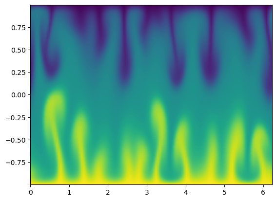
plt.contourf(X[1], X[0], T_.backward(), 100)
plt.show()
A complete solver implemented in a solver class can be found in
RayleighBenard2D.py.
Note that in the final solver it is also possible to use a \((y, t)\)-dependent boundary condition
for the hot wall. And the solver can also be configured to store intermediate results to
an HDF5 format that later can be visualized in, e.g., Paraview. The movie in the
beginning of this demo has been created in Paraview.
A. Pandey, J. D. Scheel and J. Schumacher. Turbulent Superstructures in Rayleigh-B’enard Convection, Nature Communications, 9(1), pp. 2118, doi: 10.1038/s41467-018-04478-0, 2018.