Demo - 3D Poisson’s equation

Authors:

Mikael Mortensen (mikaem at math.uio.no)

Date:

April 13, 2018

Summary. This is a demonstration of how the Python module shenfun can be used to solve a 3D Poisson equation in a 3D tensor product domain that has homogeneous Dirichlet boundary conditions in one direction and periodicity in the remaining two. The solver described runs with MPI without any further considerations required from the user. Spectral convergence, as shown in Figure Convergence of 3D Poisson solvers for both Legendre and Chebyshev modified basis function, is demonstrated. The demo is implemented in slightly more generic terms (more boundary conditions) in poisson3D.py, and the numerical method is is described in more detail by J. Shen [She94] and [She95].

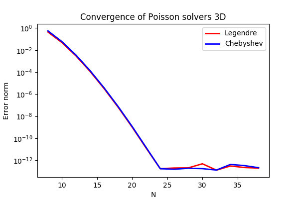
Convergence of 3D Poisson solvers for both Legendre and Chebyshev modified basis function

Poisson’s equation

Poisson’s equation is given as

(1)\[ \nabla^2 u(\boldsymbol{x}) = f(\boldsymbol{x}) \quad \text{for }\, \boldsymbol{x}=(x, y, z) \in \Omega,\]

(2)\[ u(\pm 1 ,y, z) =0,\]

(3)\[ u(x, 2\pi, z) = u(x, 0, z),\]

(4)\[ u(x, y, 2\pi) = u(x, y, 0),\]

where \(u(\boldsymbol{x})\) is the solution and \(f(\boldsymbol{x})\) is a function. The domain \(\Omega = (-1, 1)\times [0, 2\pi)^2\).

To solve Eq. (1) with the Galerkin method we will make use of smooth basis functions, \(v(\boldsymbol{x})\), that satisfy the given boundary conditions. To this end we will use one basis function for the \(x\)-direction, \(\mathcal{X}(x)\), one for the \(y\)-direction, \(\mathcal{Y}(y)\), and one for the \(z\)-direction, \(\mathcal{Z}(z)\). And then we create three-dimensional basis functions like

\[v(x, y, z) = \mathcal{X}(x) \mathcal{Y}(y) \mathcal{Z} (z).\]

The basis functions \(\mathcal{Y}(y)\) and \(\mathcal{Z}(z)\) are chosen as Fourier exponentials, since these functions are periodic. Likewise, the basis functions \(\mathcal{X}(x)\) are chosen as modified Legendre or Chebyshev polynomials, using \(\phi_l(x)\) to refer to either one

(5)\[ \mathcal{X}_l(x) = \phi_l(x) - \phi_{l+2}(x), \forall \, l \in \boldsymbol{l}^{N_0},\]

(6)\[ \mathcal{Y}_m(y) = e^{\imath m y}, \forall \, m \in \boldsymbol{m}^{N_1},\]

(7)\[ \mathcal{Z}_n(z) = e^{\imath n z}, \forall \, n \in \boldsymbol{n}^{N_2},\]

where the size of the discretized problem is \(\boldsymbol{N} = (N_0, N_1, N_2)\), \(\boldsymbol{l}^{N_0} = (0, 1, \ldots, N_0-3)\), \(\boldsymbol{m}^{N_1} = (-N_1/2, -N_1/2+1, \ldots, N_1/2-1)\) and \(\boldsymbol{n}^{N_2} = (-N_2/2, -N_2/2+1, \ldots, N_2/2-1)\). However, due to Hermitian symmetry, we only store \(N_2/2+1\) wavenumbers in the \(z\)-direction, such that \(\boldsymbol{n}^{N_2} = (0, 1, \ldots, N_2/2)\). We refer to the Cartesian wavenumber mesh on vector form as \(\boldsymbol{k}\):

\[\boldsymbol{k} = \{(l, m, n)\, | \,(l, m, n) \in \boldsymbol{l}^{N_0} \times \boldsymbol{m}^{N_1} \times \boldsymbol{n}^{N_2}\}.\]

We have the one-dimensional spaces

(8)\[ V^{N_0} = \text{span}\{ \mathcal{X}_l \}_{l\in\boldsymbol{l}^{N_0}},\]

(9)\[ V^{N_1} = \text{span}\{ \mathcal{Y}_m \}_{m\in\boldsymbol{m}^{N_1}},\]

(10)\[ V^{N_2} = \text{span}\{ \mathcal{Z}_n \}_{n\in\boldsymbol{n}^{N_2}},\]

and from these we create a tensor product space \(W^{\boldsymbol{N}}(\boldsymbol{x})\)

(11)\[ W^{\boldsymbol{N}}(\boldsymbol{x}) = V^{N_0}(x) \otimes V^{N_1}(y) \otimes V^{N_2}(z).\]

And then we look for discrete solutions \(u \in W^{\boldsymbol{N}}\) like

(12)\[ u(\boldsymbol{x}) = \sum_{l\in \boldsymbol{l}^{N_0}} \sum_{m\in \boldsymbol{m}^{N_1}}\sum_{n\in \boldsymbol{n}^{N_2}}\hat{u}_{lmn} \mathcal{X}_l(x) \mathcal{Y}_m(y) \mathcal{Z}_n(z),\]

(13)\[ = \sum_{\boldsymbol{\textsf{k}} \in \boldsymbol{k}}\hat{u}_{\boldsymbol{\textsf{k}}} v_{\boldsymbol{\textsf{k}}}(\boldsymbol{x}),\]

where \(\hat{u}_{lmn}\) are components of the expansion coefficients for \(u\) and the second form, \(\{\hat{u}_{\boldsymbol{\textsf{k}}}\}_{\boldsymbol{\textsf{k}}\in\boldsymbol{k}}\), is a shorter, simplified notation, with sans-serif \(\boldsymbol{\textsf{k}}=(l, m, n)\). The expansion coefficients are the unknowns in the spectral Galerkin method.

We now formulate a variational problem using the Galerkin method: Find \(u \in W^{\boldsymbol{N}}\) such that

(14)\[ \int_{\Omega} \nabla^2 u \, \overline{v} \, w\, \boldsymbol{dx} = \int_{\Omega} f \, \overline{v}\, w\, \boldsymbol{dx} \quad \forall v \, \in \, W^{\boldsymbol{N}}.\]

Here \(\boldsymbol{dx}=dxdydz\), and the overline represents a complex conjugate, which is needed here because the Fourier exponentials are complex functions. The weighted integrals, weighted by \(w(\boldsymbol{x})\), are called inner products, and a common notation is

(15)\[ \int_{\Omega} u \, \overline{v} \, w\, \boldsymbol{dx} = \langle u, v\rangle _w.\]

The integral can either be computed exactly, or with quadrature. The advantage of the latter is that it is faster (through Fast Fourier transforms), and that non-linear terms may be computed just as quickly as linear. For a linear problem, it does not make much of a difference, if any at all. Approximating the integral with quadrature, we obtain

\[\begin{split}\begin{align*} \int_{\Omega} u \, \overline{v} \, w\, \boldsymbol{dx} &\approx \langle u, v \rangle_w^{\boldsymbol{N}}, \\ &\approx \sum_{i=0}^{N_0-1} \sum_{j=0}^{N_1-1}\sum_{k=0}^{N_2-1} u(x_i, y_j, z_k) \overline{v}(x_i, y_j, z_k) w(x_i, y_j, z_k), \end{align*}\end{split}\]

where \(w(\boldsymbol{x})\) now are the quadrature weights. The quadrature points \(\{x_i\}_{i=0}^{N_0-1}\) are specific to the chosen basis, and even within basis there are two different choices based on which quadrature rule is selected, either Gauss or Gauss-Lobatto. The quadrature points for the Fourier bases are simply uniformly distributed throughout the domain.

Inserting for test function (12) and trialfunction \(v_{pqr} = \mathcal{X}_{p} \mathcal{Y}_q \mathcal{Z}_r\) on the left hand side of (14), we get (with summation on repeated indices to avoid too much clutter)

\[\begin{split}\begin{align*} \langle \nabla^2u, v \rangle_w^{\boldsymbol{N}} &= \left\langle \nabla^2\sum_{l\in \boldsymbol{l}^{N_0}} \sum_{m\in \boldsymbol{m}^{N_1}}\sum_{n\in \boldsymbol{n}^{N_2}}\hat{u}_{lmn} \mathcal{X}_{l} \mathcal{Y}_m \mathcal{Z}_n, \mathcal{X}_{p} \mathcal{Y}_q \mathcal{Z}_r \right\rangle_w^{\boldsymbol{N}}, \\ &= \left[\left(\mathcal{X}_l^{''}, \mathcal{X}_p \right)_w^N - (m^2+n^2)\left(\mathcal{X}_l, \mathcal{X}_p \right)_w^N \right]\delta_{mq} \delta_{nr} \hat{u}_{lmn}, \\ &= \left( a_{pl} - (m^2 + n^2)b_{pl}\right) \hat{u}_{lqr}, \quad \forall (p,q,r) \in \boldsymbol{k}, \end{align*}\end{split}\]

where the notation \((\cdot, \cdot)_w^{N_0}\)

(16)\[ b_{pl} = \left( \mathcal{X}_l, \mathcal{X}_p \right)_w^{N_0} = \sum_{i=0}^{N_0-1} \mathcal{X}_l(x_i) \mathcal{X}_p(x_i) w(x_i),\]

is used to represent a discrete \(L_2\) inner product along only the first, nonperiodic, direction. The delta functions above come from integrating over the two periodic directions, where we use constant weight functions \(w=1/(2\pi)\) in the inner products

(17)\[ \int_0^{2\pi} \mathcal{Y}_m(y) \overline{\mathcal{Y}}_q(y) \frac{1}{2\pi} dy = \delta_{mq},\]

(18)\[ \int_0^{2\pi} \mathcal{Z}_n(z) \overline{\mathcal{Z}}_r(z) \frac{1}{2\pi} dz = \delta_{nr}.\]

The Kronecker delta-function \(\delta_{ij}\) is one for \(i=j\) and zero otherwise.

The right hand side of Eq. (14) is computed as

(19)\[ \tilde{f}_{pqr} = \left\langle f, \mathcal{X}_{p} \mathcal{Y}_q \mathcal{Z}_r \right \rangle_w^{\boldsymbol{N}},\]

where a tilde is used because this is not a complete transform of the function \(f\), but only an inner product.

The linear system of equations to solve for the expansion coefficients can now be found as follows

(20)\[ \left(a_{lp} - (m^2+n^2)b_{lp}\right) \hat{u}_{pmn} = \tilde{f}_{lmn}\quad \forall \, (l,m,n) \in \boldsymbol{k}.\]

Now, when \(\hat{\boldsymbol{u}} = \{\hat{u}_{\boldsymbol{\textsf{k}}}\}_{\boldsymbol{\textsf{k}} \in \boldsymbol{k}}\) is found by solving this linear system over the entire computational mesh, it may be transformed to real space \(u(\boldsymbol{x})\) using (12). Note that the matrices \(A \in \mathbb{R}^{N_0-2 \times N_0-2}\) and \(B \in \mathbb{R}^{N_0-2 \times N_0-2}\) differ for Legendre or Chebyshev bases, but for either case they have a special structure that allows for a solution to be found very efficiently in the order of \(\mathcal{O}(N_0-3)\) operations given \(m\) and \(n\), see [She94] and [She95]. Fast solvers for (20) are implemented in shenfun for both bases.

Method of manufactured solutions

In this demo we will use the method of manufactured solutions to demonstrate spectral accuracy of the shenfun bases. To this end we choose a smooth analytical function that satisfies the given boundary conditions:

(21)\[ u_e(x, y, z) = \left(\cos(4x) + \sin(2y) + \sin(4z)\right)(1-x^2).\]

Sending \(u_e\) through the Laplace operator, we obtain the right hand side

(22)\[ \nabla^2 u_e(x,y,z) = -16(1 - x^2) \cos(4 x) + 16 x \sin(4 x) - 2 \cos(4 x) - (1-x^2)(4 \sin(2y) + 16\sin(4z)).\]

Now, setting \(f_e(\boldsymbol{x}) = \nabla^2 u_e(\boldsymbol{x})\) and solving for \(\nabla^2 u(\boldsymbol{x}) = f_e(\boldsymbol{x})\), we can compare the numerical solution \(u(\boldsymbol{x})\) with the analytical solution \(u_e(\boldsymbol{x})\) and compute error norms.

Implementation

Preamble

We will solve the Poisson problem using the shenfun Python module. The first thing needed is then to import some of this module’s functionality plus some other helper modules, like Numpy and Sympy:

from sympy import symbols, cos, sin, exp, lambdify
import numpy as np
from shenfun.tensorproductspace import TensorProductSpace
from shenfun import inner, div, grad, TestFunction, TrialFunction, Function, \
    project, Dx, FunctionSpace, comm, Array, chebyshev, dx, la

We use Sympy for the manufactured solution and Numpy for testing. MPI for Python (mpi4py) is required for running the solver with MPI.

Manufactured solution

The exact solution \(u_e(x, y, z)\) and the right hand side \(f_e(x, y, z)\) are created using Sympy as follows

x, y, z = symbols("x,y,z")
ue = (cos(4*x) + sin(2*y) + sin(4*z))*(1-x**2)
fe = ue.diff(x, 2) + ue.diff(y, 2) + ue.diff(z, 2)

These solutions are now valid for a continuous domain. The next step is thus to discretize, using the computational mesh

\[(x_i, y_j, z_k)\, \forall \, (i, j, k) \in [0, 1,\ldots, N_0-1] \times [0, 1, \ldots, N_1-1] \times [0, 1, \ldots, N_2-1]\]

and a finite number of basis functions.

Note that it is not mandatory to use Sympy for the manufactured solution. Since the solution is known (22), we could just as well simply use Numpy to compute \(f_e\). However, with Sympy it is much easier to experiment and quickly change the solution.

Discretization and MPI

We create three function spaces with given size, one for each dimension of the problem. From these three spaces a TensorProductSpace is created.

# Size of discretization
N = [14, 15, 16]

SD = FunctionSpace(N[0], 'Chebyshev', bc=(0, 0))
#SD = FunctionSpace(N[0], 'Legendre', bc=(0, 0))
K1 = FunctionSpace(N[1], 'Fourier', dtype='D')
K2 = FunctionSpace(N[2], 'Fourier', dtype='d')
T = TensorProductSpace(comm, (SD, K1, K2), axes=(0, 1, 2))
X = T.local_mesh()

Note that we can either choose a Legendre or a Chebyshev basis for the nonperiodic direction. The TensorProductSpace class takes an MPI communicator as first argument and the computational mesh is distributed internally using the pencil method. The T.local_mesh method returns the mesh local to each processor. The axes keyword determines the order of transforms going back and forth between real and spectral space. With axes=(0, 1, 2) and a forward transform (from real space to spectral, i.e., from \(u\) to \(\hat{u}\)) axis 2 is transformed first and then 1 and 0, respectively.

The manufactured solution is created with Dirichlet boundary conditions in the \(x\)-direction, and for this reason SD is the first space in T. We could just as well have put the nonperiodic direction along either \(y\)- or \(z\)-direction, though, but this would then require that the order of the transformed axes be changed as well. For example, putting the Dirichlet direction along \(y\), we would need to create the tensorproductspace as

T = TensorProductSpace(comm, (K1, SD, K2), axes=(1, 0, 2))

such that the Dirichlet direction is the last to be transformed. The reason for this is that only the Dirichlet direction leads to matrices that need to be inverted (or solved). And for this we need the entire data array along the Dirichlet direction to be local to the processor. If the SD basis is the last to be transformed, then the data will be aligned in this direction, whereas the other two directions may both, or just one of them, be distributed.

Note that X is a list containing local values of the arrays \(\{x_i\}_{i=0}^{N_0-1}\), \(\{y_j\}_{j=0}^{N_1-1}\) and \(\{z_k\}_{k=0}^{N_2-1}\). Now, it’s not possible to run a jupyter notebook with more than one process, but we can imagine running the complete solver with 4 procesors and a processor mesh of shape \(2\times 2\). We would then get the following local slices for each processor in spectral space

print(comm.Get_rank(), T.local_slice())
3 [slice(0, 14, None), slice(8, 15, None), slice(5, 9, None)]
1 [slice(0, 14, None), slice(0, 8, None), slice(5, 9, None)]
2 [slice(0, 14, None), slice(8, 15, None), slice(0, 5, None)]
0 [slice(0, 14, None), slice(0, 8, None), slice(0, 5, None)]

where the global shape is \(\boldsymbol{N}=(14, 15, 9)\) after taking advantage of Hermitian symmetry in the \(z\)-direction. So, all processors have the complete first dimension available locally, as they should. Furthermore, processor three owns the slices from \(8:15\) and \(5:9\) along axes \(y\) and \(z\), respectively. Processor 2 owns slices \(0:8\) and \(0:5\) etc. In real space the mesh is distributed differently. First of all the global mesh shape is \(\boldsymbol{N}=(14, 15, 16)\), and it is distributed along the first two dimensions. The local slices can be inspected as

print(comm.Get_rank(), T.local_slice(False))
0 [slice(0, 7, None), slice(0, 8, None), slice(0, 16, None)]
1 [slice(0, 7, None), slice(8, 15, None), slice(0, 16, None)]
2 [slice(7, 14, None), slice(0, 8, None), slice(0, 16, None)]
3 [slice(7, 14, None), slice(8, 15, None), slice(0, 16, None)]

Since two directions are distributed, both in spectral and real space, we say that we have a two-dimensional decomposition (here a \(2\times 2\) shaped processor mesh) and the MPI distribution is of type pencil. It is also possible to choose a slab decomposition, where only one dimension of the array is distributed. This choice needs to be made when creating the tensorproductspace as

T = TensorProductSpace(comm, (SD, K1, K2), axes=(0, 1, 2), slab=True)

which would lead to a mesh that is distributed along \(x\)-direction in real space and \(y\)-direction in spectral space. The local slices would then be

print(comm.Get_rank(), T.local_slice()) # spectral space
1 [slice(0, 14, None), slice(4, 8, None), slice(0, 9, None)]
2 [slice(0, 14, None), slice(8, 12, None), slice(0, 9, None)]
0 [slice(0, 14, None), slice(0, 4, None), slice(0, 9, None)]
3 [slice(0, 14, None), slice(12, 15, None), slice(0, 9, None)]
print(comm.Get_rank(), T.local_slice(False)) # real space
3 [slice(11, 14, None), slice(0, 15, None), slice(0, 16, None)]
0 [slice(0, 4, None), slice(0, 15, None), slice(0, 16, None)]
2 [slice(8, 11, None), slice(0, 15, None), slice(0, 16, None)]
1 [slice(4, 8, None), slice(0, 15, None), slice(0, 16, None)]

Note that the slab decomposition is usually the fastest choice. However, the maximum number of processors with slab is \(\min \{N_0, N_1\}\), whereas a pencil approach can be used with up to \(\min \{N_1(N_2/2+1), N_0 N_1\}\) processors.

Variational formulation

The variational problem (14) can be assembled using shenfun’s form language, which is perhaps surprisingly similar to FEniCS.

u = TrialFunction(T)
v = TestFunction(T)
# Get f on quad points
fj = Array(T, buffer=fe)
# Compute right hand side of Poisson equation
f_hat = inner(v, fj)
# Get left hand side of Poisson equation
matrices = inner(v, div(grad(u)))

The Laplacian operator is recognized as div(grad). The matrices object is a list of two tensor product matrices, stored as instances of the class TPMatrix. The two tensor product matrices represents

\[a_{pl} \delta_{mq} \delta_{nr}\, \text{ and }\, -(m^2 + n^2)b_{pl} \delta_{mq} \delta_{nr}\]

from Eqs. (20), (17) and (18). The second matrix (\(-(m^2 + n^2)b_{pl} \delta_{mq} \delta_{nr}\)) has an attribute scale that is equal to \(-(m^2+n^2)\). This scale is stored as a numpy array of shape \((1, 15, 9)\), representing the set \(\{-(m^2+n^2): (m, n) \in \boldsymbol{m}^{N_1} \times \boldsymbol{n}^{N_2}\}\). Note that \(\boldsymbol{n}^{N_2}\) is stored simply as an array of length \(N_2/2+1\) (here 9), since the transform in direction \(z\) takes a real signal and transforms it taking advantage of Hermitian symmetry, see rfft.

Solve linear equations

Finally, solve linear equation system and transform solution from spectral \(\hat{u}_{\boldsymbol{\textsf{k}}}\) vector to the real space \(u(\boldsymbol{x})\) and then check how the solution corresponds with the exact solution \(u_e\).

# Create Helmholtz linear algebra solver
Solver = chebyshev.la.Helmholtz
#Solver = la.SolverGeneric1ND # For Legendre
H = Solver(matrices)

# Solve and transform to real space
u_hat = Function(T)           # Solution spectral space
u_hat = H(u_hat, f_hat)       # Solve
uq = T.backward(u_hat)

# Compare with analytical solution
uj = Array(T, buffer=ue)
error = comm.reduce(np.linalg.norm(uj-uq)**2)
if comm.Get_rank() == 0:
    print("Error=%2.16e" %(np.sqrt(error)))

Convergence test

To do a convergence test we will now create a function main, that takes the number of quadrature points as parameter, and prints out the error.

def main(N, family='Chebyshev'):
    Solver = chebyshev.la.Helmholtz if family.lower() == 'chebyshev' else la.SolverGeneric1ND
    SD = FunctionSpace(N, family=family, bc=(0, 0))
    K1 = FunctionSpace(N, family='F', dtype='D')
    K2 = FunctionSpace(N, family='F', dtype='d')
    T = TensorProductSpace(comm, (SD, K1, K2), axes=(0, 1, 2))

    u = TrialFunction(T)
    v = TestFunction(T)

    # Get f on quad points
    fj = Array(T, buffer=fe)

    # Compute right hand side of Poisson's equation
    f_hat = Function(T)
    f_hat = inner(v, fj, output_array=f_hat)
    if family == 'legendre':
        f_hat *= -1.

    # Get left hand side of Poisson equation
    if family.lower() == 'chebyshev':
        matrices = inner(v, div(grad(u)))
    else:
        matrices = inner(grad(v), grad(u))

    # Create Helmholtz linear algebra solver
    H = Solver(matrices)

    # Solve and transform to real space
    u_hat = Function(T)           # Solution spectral space
    u_hat = H(f_hat, u_hat)       # Solve

    uj = Array(T)
    uj = u_hat.backward(uj)

    # Compare with analytical solution
    ua = Array(T, buffer=ue)
    #l2_error = np.linalg.norm(uj-ua)
    L2_error = np.sqrt(dx((uj-ua)**2))
    return L2_error

For example, we find the error of a Chebyshev discretization using 12 quadrature points as

main(12, 'Chebyshev')

To get the convergence we call main for a list of \(N=[12, 16, \ldots, 48]\), and collect the errornorms in arrays to be plotted. The error can be plotted using matplotlib, and the generated figure is also shown in this demos summary.

import matplotlib.pyplot as plt

N = range(12, 50, 4)
error = {}
for basis in ('legendre', 'chebyshev'):
    error[basis] = []
    for i in range(len(N)):
        errN = main(N[i], basis)
        error[basis].append(errN)

plt.figure(figsize=(6, 4))
for basis, col in zip(('legendre', 'chebyshev'), ('r', 'b')):
    plt.semilogy(N, error[basis], col, linewidth=2)
plt.title('Convergence of Poisson solvers 1D')
plt.xlabel('N')
plt.ylabel('Error norm')
plt.legend(('Legendre', 'Chebyshev'))
plt.show()

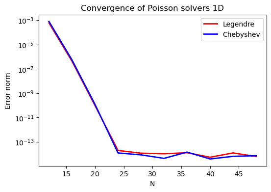
The spectral convergence is evident and we can see that after \(N=24\) roundoff errors dominate as the errornorm trails off around \(10^{-14}\).

Complete solver

A complete solver, that can use any family of bases (Chebyshev, Legendre, Jacobi, Chebyshev second kind), and any kind of boundary condition, can be found here.