Getting started

Basic usage

Shenfun consists of classes and functions whoose purpose it is to make it easier to implement PDE’s with spectral methods in simple tensor product domains. The most important everyday tools are

• TensorProductSpace

• CompositeSpace

• TrialFunction

• TestFunction

• Function

• Array

• inner()

• div()

• grad()

• project()

• FunctionSpace()

A good place to get started is by creating a FunctionSpace(). There are eight families of function spaces: Fourier, Chebyshev (first and second kind), Legendre, Laguerre, Hermite, Ultraspherical and Jacobi. All spaces are defined on a one-dimensional reference domain, with their own basis functions and quadrature points. For example, we have the regular orthogonal Chebyshev space \(\text{span}\{T_k\}_{k=0}^{N-1}\), where \(T_k\) is the \(k\)’th Chebyshev polynomial of the first kind. To create such a function space with 8 quadrature points do:

from shenfun import FunctionSpace
N = 8
T = FunctionSpace(N, 'Chebyshev', bc=None)

Here bc=None is used to indicate that there are no boundary conditions associated with this space, which is the default, so it could just as well have been left out. To create a regular orthogonal Legendre function space (i.e., \(\text{span}\{L_k\}_{k=0}^{N-1}\), where \(L_k\) is the \(k\)’th Legendre polynomial), just replace Chebyshev with Legendre above. And to create a Fourier function space, just use Fourier.

The function space \(T = \text{span}\{T_k\}_{k=0}^{N-1}\) has many useful methods associated with it, and we may experiment a little. A Function u using the basis in \(T\) has expansion

(1)\[ u(x) = \sum_{k=0}^{N} \hat{u}_k T_k(x)\]

and an instance of this function (initialized with \(\hat{u}_k=0, \, k = 0, 1, \ldots, N\)) is created in shenfun as:

from shenfun import Function
u = Function(T)

Consider now for example the polynomial \(u_e(x)=2x^2-1\), which happens to be exactly equal to \(T_2(x)\). We can create this polynomial using sympy

import sympy as sp
x = sp.Symbol('x')
ue = 2*x**2 - 1  # or simply ue = sp.chebyshevt(2, x)

The Sympy function ue can now be evaluated on the quadrature points of basis \(T\):

from shenfun import Array
xj = T.mesh()
ua = Array(T)
ua[:] = [ue.subs(x, xx) for xx in xj]
print(xj)
  [ 0.98078528  0.83146961  0.55557023  0.19509032 -0.19509032 -0.55557023
   -0.83146961 -0.98078528]
print(ua)
  [ 0.92387953  0.38268343 -0.38268343 -0.92387953 -0.92387953 -0.38268343
    0.38268343  0.92387953]

We see that ua is an Array on the function space T, and not a Function. The Array and Function classes are both subclasses of Numpy’s ndarray, and represent the two arrays associated with a spectral Galerkin function, like (1). The Function represents the entire spectral Galerkin function, with array values corresponding to the sequence of expansion coefficients \(\boldsymbol{\hat{u}}=\{\hat{u}_k\}_{k=0}^{7}\). The Array represents the spectral Galerkin function evaluated on the quadrature mesh of the function space T, which here is equal to \(\{u_e(x_i)\}_{i=0}^7\).

We now want to find the Function uh corresponding to Array ua. Considering (1), this corresponds to finding \(\boldsymbol{\hat{u}}\) if the left hand side \(u(x_j)\) is known for all quadrature points \(x_j\).

Since we already know that ue(x) is equal to the second Chebyshev polynomial, we should get an array of expansion coefficients equal to \(\boldsymbol{\hat{u}} = (0, 0, 1, 0, 0, 0, 0, 0)\). We can compute uh either by using project() or a forward transform:

from shenfun import project
uh = Function(T)
uh = T.forward(ue, uh)
# or
# uh = ue.forward(uh)
# or
# uh = project(ue, T)
print(uh)
  [-1.38777878e-17  6.72002101e-17  1.00000000e+00 -1.95146303e-16
    1.96261557e-17  1.15426347e-16 -1.11022302e-16  1.65163507e-16]

So we see that the projection works to machine precision.

The projection is mathematically: find \(u_h \in T\), such that

\[(u_h - u_e, v)_w = 0 \quad \forall v \in T,\]

where \(v\) is a test function, \(u_h\) is a trial function and the notation \((\cdot, \cdot)_w\) was introduced in (4). Using now \(v=T_k\) and \(u_h=\sum_{j=0}^7 \hat{u}_j T_j\), we get

\[\begin{split}(\sum_{j=0}^7 \hat{u}_j T_j, T_k)_w &= (u_e, T_k)_w, \\ \sum_{j=0}^7 (T_j, T_k)_w \hat{u}_j &= (u_e, T_k)_w,\end{split}\]

for \(k = 0, 1, \ldots, 7\). This can be rewritten on matrix form as

\[b_{kj} \hat{u}_j = \tilde{u}_k,\]

where \(b_{kj} = (T_j, T_k)_w\), \(\tilde{u}_k = (u_e, T_k)_w\) and summation is implied by the repeating \(j\) indices. Since the Chebyshev polynomials are orthogonal the mass matrix \(B=(b_{kj}) \in \mathbb{R}^{N \times N}\) is diagonal. We can assemble both the matrix \(B\) and the vector \(\boldsymbol{\tilde{u}}=(\tilde{u}_j) \in \mathbb{R}^N\) with shenfun, and at the same time introduce the TestFunction, TrialFunction classes and the inner() function:

from shenfun import TestFunction, TrialFunction, inner
u = TrialFunction(T)
v = TestFunction(T)
B = inner(u, v)
u_tilde = inner(ue, v)
dict(B)
  {0: array([3.14159265, 1.57079633, 1.57079633, 1.57079633, 1.57079633,
   1.57079633, 1.57079633, 1.57079633])}
print(u_tilde)
  [-4.35983562e-17  1.05557843e-16  1.57079633e+00 -3.06535096e-16
    3.08286933e-17  1.81311282e-16 -1.74393425e-16  2.59438230e-16]

The inner() function represents the (weighted) inner product and it expects one test function, and possibly one trial function. If, as here, it also contains a trial function, then a matrix is returned. If inner() contains one test, but no trial function, then an array is returned. Finally, if inner() contains no test nor trial function, but instead a number and an Array, like:

a = Array(T, val=1)
print(inner(1, a))
  2.0

then inner() represents a non-weighted integral over the domain. Here it returns the length of the domain (2.0) since a is initialized to unity.

Note that the matrix \(B\) assembled above is stored using shenfun’s SpectralMatrix class, which is a subclass of Python’s dictionary, where the keys are the diagonals and the values are the diagonal entries. The matrix \(B\) is seen to have only one diagonal (the principal) \((b_{ii})_{i=0}^{7}\).

With the matrix comes a solve method and we can solve for \(\hat{u}\) through:

u_hat = Function(T)
u_hat = B.solve(u_tilde, u=u_hat)
print(u_hat)
  [-1.38777878e-17  6.72002101e-17  1.00000000e+00 -1.95146303e-16
    1.96261557e-17  1.15426347e-16 -1.11022302e-16  1.65163507e-16]

which obviously is exactly the same as we found using project() or the T.forward function.

Note that Array merely is a subclass of Numpy’s ndarray, whereas Function is a subclass of both Numpy’s ndarray and the BasisFunction class. The latter is used as a base class for arguments to bilinear and linear forms, and is as such a base class also for TrialFunction and TestFunction. An instance of the Array class cannot be used in forms, except from regular inner products of numbers or test function vs an Array. To illustrate, lets create some forms, where all except the last one is ok:

from shenfun import Dx
T = FunctionSpace(12, 'Legendre')
u = TrialFunction(T)
v = TestFunction(T)
uf = Function(T)
ua = Array(T)
A = inner(v, u)   # Mass matrix
c = inner(v, ua)  # ok, a scalar product
d = inner(v, uf)  # ok, a scalar product (slower than above)
e = inner(1, ua)  # ok, non-weighted integral of ua over domain
df = Dx(uf, 0, 1) # ok
da = Dx(ua, 0, 1) # Not ok

    AssertionError                            Traceback (most recent call last)
    <ipython-input-14-3b957937279f> in <module>
    ----> 1 da = inner(v, Dx(ua, 0, 1))

    ~/MySoftware/shenfun/shenfun/forms/operators.py in Dx(test, x, k)
         82         Number of derivatives
         83     """
    ---> 84     assert isinstance(test, (Expr, BasisFunction))
         85
         86     if isinstance(test, BasisFunction):

    AssertionError:

So it is not possible to perform operations that involve differentiation (Dx represents a partial derivative) on an Array instance. This is because the ua does not contain more information than its values and its TensorProductSpace. A BasisFunction instance, on the other hand, can be manipulated with operators like div() grad() in creating instances of the Expr class, see Operators.

Note that any rules for efficient use of Numpy ndarrays, like vectorization, also applies to Function and Array instances.

Operators

Operators act on any single instance of a BasisFunction, which can be Function, TrialFunction or TestFunction. The implemented operators are:

• div()

• grad()

• curl()

• Dx()

Operators are used in variational forms assembled using inner() or project(), like:

A = inner(grad(u), grad(v))

which assembles a stiffness matrix A. Note that the two expressions fed to inner must have consistent rank. Here, for example, both grad(u) and grad(v) have rank 1 of a vector.

Boundary conditions

The FunctionSpace() has a keyword bc that can be used to specify boundary conditions. This keyword can take several different inputs. The default is None, which will return an orthogonal space with no boundary condition associated. This means for example a pure orthogonal Chebyshev or Legendre series, if these are the families. Otherwise, a Dirichlet space can be chosen using either one of:

bc = (a, b)
bc = {'left': {'D': a}, 'right': {'D': b}}
bc = f"u(-1)={a} && u(1)={b}"

This sets a Dirichlet boundary condition on both left and right hand side of the domain, with a and b being the values. The third option uses the location of the boundary, so here the domain is the standard reference domain (-1, 1). Similarly, a pure Neumann space may be chosen using either:

bc = {'left': {'N': a}, 'right': {'N': b}}
bc = f"u'(-1)={a} && u'(1)={b}"

Using either one of:

bc = (None, b)
bc = {'right': {'D': b}}
bc = f"u(1)={b}"

returns a space with only one Dirichlet boundary condition, on the right hand side of the domain. For one Dirichlet boundary condition on the left instead use bc = (a, None), bc = {'left': {'D': a}} or bc = f"u(-1)={a}".

Using either one of:

bc = (a, b, c, d)
bc = {'left': {'D': a, 'N': b}}, 'right': {'D': c, 'N': d}}
bc = f"u({-1})={a} && u'(-1)={b} && u(1)={c} && u'(1)={d}"

returns a space with 4 boundary conditions (biharmonic), where a and b are the Dirichlet and Neumann values on the left boundary, whereas c and d are the values on right.

The Laguerre basis is used to solve problems on the half-line \(x \in [0, \infty)\). For this family you can only specify boundary conditions at the left boundary. However, the Poisson equation requires only one condition, and the biharmonic problem two. The solution is automatically set to zero at \(x \rightarrow \infty\).

Any kind of boundary condition may be specified. For higher order derivatives, use the form bc = f"u''(-1)={a}", or bc = {'left': {'N2': a}}, and similar for higher order.

Multidimensional problems

As described in the introduction, a multidimensional problem is handled using tensor product spaces, that have basis functions generated from taking the outer products of one-dimensional basis functions. We create tensor product spaces using the class TensorProductSpace:

N, M = (12, 16)
C0 = FunctionSpace(N+2, 'L', bc=(0, 0), scaled=True)
K0 = FunctionSpace(M, 'F', dtype='d')
T = TensorProductSpace(comm, (C0, K0))

Associated with this is a Cartesian domain \([-1, 1] \times [0, 2\pi)\). We use classes Function, TrialFunction and TestFunction exactly as before:

u = TrialFunction(T)
v = TestFunction(T)
A = inner(grad(u), grad(v))

However, now A will be a tensor product matrix, or more correctly, the sum of two tensor product matrices. This can be seen if we look at the equations beyond the code. In this case we are using a composite Legendre basis for the first direction and Fourier exponentials for the second, and the tensor product basis function is

\[\begin{split}v_{kl}(x, y) &= \frac{1}{\sqrt{4k+6}}(L_k(x) - L_{k+2}(x)) \exp(\imath l y), \\ &= \psi_k(x) \exp(\imath l y),\end{split}\]

where \(\imath=\sqrt{-1}\), \(L_k\) is the \(k\)’th Legendre polynomial and \(\psi_k = (L_k-L_{k+2})/\sqrt{4k+6}\) is used for simplicity in later expressions. The trial function is now

\[u(u, y) = \sum_{k=0}^{N-1} \sum_{l=-M/2}^{M/2-1} \hat{u}_{kl} \psi_k(x) \exp(\imath l y)\]

where the sum on the Fourier exponentials will be implemented to take advantage of the Hermitian symmetry of the real input data. That is, \(\hat{u}_{k,l} = \overline{\hat{u}}_{k,-l}\), where the overline represents a complex conjugate. Note that because of this symmetry the shape of the stored array \((\hat{u}_{kl})\) will be \(N \times M/2+1\).

The inner product (inner(grad(u), grad(v))) is now computed as

(2)\[\begin{split}(\nabla u, \nabla v)_w &= \int_{-1}^{1} \int_{0}^{2 \pi} \nabla u \cdot \nabla \overline{v} \omega dxdy, \\ &= \frac{1}{2\pi} \int_{-1}^{1} \int_{0}^{2 \pi} \left(\frac{\partial u}{\partial x} \frac{\partial \overline{v}}{\partial x} + \frac{\partial u}{\partial y}\frac{\partial \overline{v}}{\partial y}\right) dxdy, \\ &= \frac{1}{2\pi} \int_{-1}^{1} \int_{0}^{2 \pi} \frac{\partial u}{\partial x} \frac{\partial \overline{v}}{\partial x} dxdy + \frac{1}{2\pi} \int_{-1}^{1} \int_{0}^{2 \pi} \frac{\partial u}{\partial y} \frac{\partial \overline{v}}{\partial y} dxdy,\end{split}\]

where \(\overline{v}\) is the complex conjugate of \(v\) and we use the weight \(\omega = 1/2\pi\). We see that the inner product is really the sum of two tensor product matrices. However, each one of these also contains the outer product of smaller matrices. To see this we need to insert for the trial and test functions (using \(v_{mn}\) for test):

\[\begin{split}\frac{1}{2\pi}\int_{-1}^{1} &\int_{0}^{2 \pi} \frac{\partial u}{\partial x} \frac{\partial \overline{v}}{\partial x} dxdy \\ &= \frac{1}{2\pi}\int_{-1}^{1} \int_{0}^{2 \pi} \frac{\partial}{\partial x} \left( \sum_{k=0}^{N-1} \sum_{l=0}^{M/2} \hat{u}_{kl} \psi_k \exp(\imath l y) \right) \frac{\partial}{\partial x} \left(\psi_m \exp(- \imath n y)\right) dxdy, \\ &= \sum_{k=0}^{N-1} \sum_{l=-M/2}^{M/2-1} \underbrace{ \int_{-1}^{1} \frac{\partial \psi_k}{\partial x} \frac{\partial \psi_m}{\partial x} dx}_{a_{mk}} \underbrace{ \frac{1}{2\pi}\int_{0}^{2 \pi} \exp(\imath l y) \exp(-\imath n y) dy }_{b_{nl}} \, \hat{u}_{kl},\end{split}\]

where \(A = (a_{mk}) \in \mathbb{R}^{N \times N}\) and \(B = (b_{nl}) \in \mathbb{R}^{(M/2+1)\times (M/2+1)}\), again using the Hermitian symmetry to reduce the shape of the Fourier axis to \(M/2+1\). The tensor product matrix \(a_{mk} b_{nl}\) (or in matrix notation \(A \otimes B\)) is the first item of the two items in the list that is returned by inner(grad(u), grad(v)). The other item is of course the second term in the last line of (2):

\[\begin{split}\frac{1}{2\pi} \int_{-1}^{1} &\int_{0}^{2 \pi} \frac{\partial u}{\partial y} \frac{\partial \overline{v}}{\partial y} dxdy \\ &= \frac{1}{2\pi}\int_{-1}^{1} \int_{0}^{2 \pi} \frac{\partial}{\partial y} \left( \sum_{k=0}^{N-1} \sum_{l=0}^{M/2} \hat{u}_{kl} \psi_k \exp(\imath l y) \right) \frac{\partial}{\partial y} \left(\psi_m \exp(- \imath n y) \right) dxdy \\ &= \sum_{k=0}^{N-1} \sum_{l=-M/2}^{M/2-1} \underbrace{ \int_{-1}^{1} \psi_k \psi_m dx}_{c_{mk}} \underbrace{\frac{1}{2\pi} \int_{0}^{2 \pi} \frac{\partial \exp(\imath l y)}{\partial y} \frac{ \partial \exp(- \imath n y) }{\partial y} dy}_{d_{nl}} \, \hat{u}_{kl}\end{split}\]

The tensor product matrices \(a_{mk} b_{nl}\) and \(c_{mk}d_{nl}\) are both instances of the TPMatrix class. Together they lead to linear algebra systems like:

(3)\[(a_{mk}b_{nl} + c_{mk}d_{nl}) \hat{u}_{kl} = \tilde{f}_{mn},\]

where \(0 \le m < N, 0 \le n \le M/2\) and \(\tilde{f}_{mn} = (v_{mn}, f)_w\) for some right hand side \(f\), see, e.g., (11). Note that an alternative formulation here is

\[A U B^T + C U D^T = F,\]

where \(U=(\hat{u}_{kl}) \in \mathbb{R}^{N \times M/2+1}\) and \(F = (\tilde{f}_{kl}) \in \mathbb{R}^{N \times M/2+1}\) are treated as regular matrices. This formulation is utilized to derive efficient solvers for tensor product bases in multiple dimensions using the matrix decomposition method in [She94] and [She95]. In shenfun we have generic solvers for such multi-dimensional problems that make use of Kronecker product matrices and the vec operation. We have

\[\begin{split}\text{vec}(A U B^T) + \text{vec}(C U D^T) &= \text{vec}(F), \\ (A \otimes B + C \otimes D ) \text{vec}(U) &= \text{vec}(F)\end{split}\]

where \(\text{vec}(U) = (\hat{u}_{0,0}, \ldots, \hat{u}_{0,M/2}, \hat{u}_{1,0}, \ldots \hat{u}_{1,M/2}, \ldots, \ldots, \hat{u}_{N-1,0}, \ldots, \hat{u}_{N-1,M/2})^T\) is a vector obtained by flattening the row-major matrix \(U\). The generic Kronecker solvers are found in Solver2D and Solver3D for two- and three-dimensional problems.

Note that in our case the equation system (3) can be greatly simplified since three of the submatrices (\(A, B\) and \(D\)) are diagonal. Even more, two of them equal the identity matrix

\[\begin{split}a_{mk} &= \delta_{mk}, \\ b_{nl} &= \delta_{nl},\end{split}\]

whereas the last one can be written in terms of the identity (no summation on repeating indices)

\[d_{nl} = l^2\delta_{nl}.\]

Inserting for this in (3) and simplifying by requiring that \(l=n\) in the second step, we get

(4)\[\begin{split}(\delta_{mk}\delta_{nl} + l^2 c_{mk}\delta_{nl}) \hat{u}_{kl} &= \tilde{f}_{mn}, \\ (\delta_{mk} + l^2 c_{mk}) \hat{u}_{kl} &= \tilde{f}_{ml}.\end{split}\]

Now if we keep \(l\) fixed this latter equation is simply a regular linear algebra problem to solve for \(\hat{u}_{kl}\), for all \(k\). Of course, this solve needs to be carried out for all \(l\).

Note that there is a generic solver SolverGeneric1ND available for problems like (3), that have one Fourier space and one non-periodic space. Another possible solver is Solver2D, which makes no assumptions of diagonality and solves the problem using a Kronecker product matrix. Assuming there is a right hand side function f, the solver is created and used as:

from shenfun import la
solver = la.SolverGeneric1ND(A)
u_hat = Function(T)
f_tilde = inner(v, f)
u_hat = solver(f_tilde, u_hat)

For multidimensional problems it is possible to use a boundary condition that is a function of the computational coordinates. For example:

import sympy as sp
x, y = sp.symbols('x,y', real=True)
B0 = FunctionSpace(N, 'C', bc=((1-y)*(1+y), 0), domain=(-1, 1))
B1 = FunctionSpace(N, 'C', bc=(0, (1-x)*(1+x)), domain=(-1, 1))
T = TensorProductSpace(comm, (B0, B1))

uses homogeneous Dirichlet on two out of the four sides of the square domain \([-1, 1]\times [-1, 1]\), at \(x=-1\) and \(y=1\). For the side where \(y=1\), the boundary condition is \((1-x)(1+x)\). Note that only \(x\) will vary along the side where \(y=1\), which is the right hand side of the domain for B1. Also note that the boundary condition on the square domain should match in the corners, or else there will be severe Gibbs oscillations in the solution. The problem with two non-periodic directions can use the solvers Solver2D or SolverGeneric2ND, where the latter can also take one Fourier direction in a 3D problem.

Curvilinear coordinates

Shenfun can be used to solve equations using curvilinear coordinates, like polar, cylindrical and spherical coordinates. The feature was added April 2020, and is still rather experimental. The curvilinear coordinates are defined by the user, who needs to provide a map, i.e., the position vector, between new coordinates and the Cartesian coordinates. The basis functions of the new coordinates need not be orthogonal, but non-orthogonal is not widely tested so use with care. In shenfun we use non-normalized natural (covariant) basis vectors. For this reason the equations may look a little bit different than usual. For example, in cylindrical coordinates we have the position vector

(5)\[\mathbf{r} = r \cos \theta \, \mathbf{i} + r \sin \theta \,\mathbf{j} + z \,\mathbf{k},\]

where \(\mathbf{i, j, k}\) are the Cartesian unit vectors and \(r, \theta, z\) are the new coordinates. The covariant basis vectors are then

(6)\[\begin{split}\mathbf{b}_r &= \frac{\partial \mathbf{r}}{ \partial r}, \\ \mathbf{b}_{\theta} &= \frac{\partial \mathbf{r}}{ \partial \theta }, \\ \mathbf{b}_z &= \frac{\partial \mathbf{r}}{ \partial z},\end{split}\]

leading to

(7)\[\begin{split}\mathbf{b}_{r}&=\cos{\left(\theta \right)}\,\mathbf{i}+\sin{\left(\theta \right)}\,\mathbf{j}, \\ \mathbf{b}_{\theta}&=- r \sin{\left(\theta \right)}\,\mathbf{i}+r \cos{\left(\theta \right)}\,\mathbf{j}, \\ \mathbf{b}_{z}&=\mathbf{k}.\end{split}\]

We see that \(|\mathbf{b}_{\theta}| = r\) and not unity. In shenfun you can choose to use covariant basis vectors, or the more common normalized basis vectors, that are also called physical basis vectors. These are

(8)\[\begin{split}\mathbf{e}_{r}&=\cos{\left(\theta \right)}\,\mathbf{i}+\sin{\left(\theta \right)}\,\mathbf{j}, \\ \mathbf{e}_{\theta}&=- \sin{\left(\theta \right)}\,\mathbf{i}+\cos{\left(\theta \right)}\,\mathbf{j}, \\ \mathbf{e}_{z}&=\mathbf{k}.\end{split}\]

To choose there is a configuration parameter called basisvectors in the configuration file shenfun.yaml (see Configuration), that can be set to either covariant or normal.

A vector \(\mathbf{u}\) in the covariant basis is given as

(9)\[\mathbf{u} = u^r \mathbf{b}_r + u^{\theta} \mathbf{b}_{\theta} + u^{z} \mathbf{b}_z,\]

and the vector Laplacian \(\nabla^2 \mathbf{u}\) is

(10)\[\begin{split}\left( \frac{\partial^2 u^{r}}{\partial^2r}+\frac{1}{r}\frac{\partial u^{r}}{\partial r}+\frac{1}{r^{2}}\frac{\partial^2 u^{r}}{\partial^2\theta}- \frac{2}{r}\frac{\partial u^{\theta}}{\partial \theta}- \frac{1}{r^{2}}u^{r}+\frac{\partial^2 u^{r}}{\partial^2z}\right) \mathbf{b}_{r} \\+\left( \frac{\partial^2 u^{\theta}}{\partial^2r}+\frac{3}{r}\frac{\partial u^{\theta}}{\partial r}+\frac{2}{r^{3}}\frac{\partial u^{r}}{\partial \theta}+\frac{1}{r^{2}}\frac{\partial^2 u^{\theta}}{\partial^2\theta}+\frac{\partial^2 u^{\theta}}{\partial^2z}\right) \mathbf{b}_{\theta} \\+\left( \frac{\partial^2 u^{z}}{\partial^2r}+\frac{1}{r}\frac{\partial u^{z}}{\partial r}+\frac{1}{r^{2}}\frac{\partial^2 u^{z}}{\partial^2\theta}+\frac{\partial^2 u^{z}}{\partial^2z}\right) \mathbf{b}_{z}.\end{split}\]

which is slightly different from what you see in most textbooks, which are using the normalized basis vectors.

Note that once the curvilinear map has been created, shenfun’s operators div(), grad() and curl() work out of the box with no additional effort. So you do not have to implement messy equations that look like (10) directly. Take the example with cylindrical coordinates. The vector Laplacian can be implemented as:

from shenfun import *
import sympy as sp

r, theta, z = psi = sp.symbols('x,y,z', real=True, positive=True)
rv = (r*sp.cos(theta), r*sp.sin(theta), z)

N = 10
F0 = FunctionSpace(N, 'F', dtype='d')
F1 = FunctionSpace(N, 'F', dtype='D')
L = FunctionSpace(N, 'L', domain=(0, 1))
T = TensorProductSpace(comm, (L, F1, F0), coordinates=(psi, rv))
V = VectorSpace(T)
u = TrialFunction(V)
du = div(grad(u))

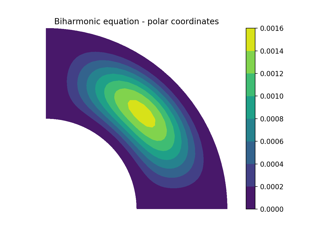
There are curvilinear demos for solving both Helmholtz’s equation and the biharmonic equation on a circular disc, a solver for 3D Poisson equation in a pipe, and a solver for the biharmonic equation on a part of the disc. Also, the Helmholtz equation solved on the unit sphere using spherical coordinates is shown here, and on the torus here. A solution from solving the biharmonic equation with homogeneous Dirichlet boundary conditions on \((\theta, r) \in [0, \pi/2] \times [0.5, 1]\) is shown below.

Coupled problems

With Shenfun it is possible to solve equations coupled and implicit using the CompositeSpace class for multidimensional problems and MixedFunctionSpace for one-dimensional problems. As an example, lets consider a mixed formulation of the Poisson equation. The Poisson equation is given as always as

(11)\[\nabla^2 u(\boldsymbol{x}) = f(\boldsymbol{x}), \quad \text{for} \quad \boldsymbol{x} \in \Omega,\]

but now we recast the problem into a mixed formulation

\[\begin{split}\sigma(\boldsymbol{x})- \nabla u (\boldsymbol{x})&= 0, \quad \text{for} \quad \boldsymbol{x} \in \Omega, \\ \nabla \cdot \sigma (\boldsymbol{x})&= f(\boldsymbol{x}), \quad \text{for} \quad \boldsymbol{x} \in \Omega.\end{split}\]

where we solve for the vector \(\sigma\) and scalar \(u\) simultaneously. The domain \(\Omega\) is taken as a multidimensional Cartesian product \(\Omega=(-1, 1) \times [0, 2\pi)\), but the code is more or less identical for a 3D problem. For boundary conditions we use Dirichlet in the \(x\)-direction and periodicity in the \(y\)-direction:

\[\begin{split}u(\pm 1, y) &= 0 \\ u(x, 2\pi) &= u(x, 0)\end{split}\]

Note that there is no boundary condition on \(\sigma\), only on \(u\). For this reason we choose a Dirichlet basis \(SD\) for \(u\) and a regular Legendre or Chebyshev \(ST\) basis for \(\sigma\). With \(K0\) representing the function space in the periodic direction, we get the relevant 2D tensor product spaces as \(TD = SD \otimes K0\) and \(TT = ST \otimes K0\). Since \(\sigma\) is a vector we use a VectorSpace \(VT = TT \times TT\) and finally a CompositeSpace \(Q = VT \times TD\) for the coupled and implicit treatment of \((\sigma, u)\):

from shenfun import VectorSpace, CompositeSpace
N, M = (16, 24)
family = 'Legendre'
SD = FunctionSpace(N[0], family, bc=(0, 0))
ST = FunctionSpace(N[0], family)
K0 = FunctionSpace(N[1], 'Fourier', dtype='d')
TD = TensorProductSpace(comm, (SD, K0), axes=(0, 1))
TT = TensorProductSpace(comm, (ST, K0), axes=(0, 1))
VT = VectorSpace(TT)
Q = CompositeSpace([VT, TD])

In variational form the problem reads: find \((\sigma, u) \in Q\) such that

(12)\[\begin{split}(\sigma, \tau)_w - (\nabla u, \tau)_w &= 0, \quad \forall \tau \in VT, \\ (\nabla \cdot \sigma, v)_w &= (f, v)_w \quad \forall v \in TD\end{split}\]

To implement this we use code that is very similar to regular, uncoupled problems. We create test and trialfunction:

gu = TrialFunction(Q)
tv = TestFunction(Q)
sigma, u = gu
tau, v = tv

and use these to assemble all blocks of the variational form (12):

# Assemble equations
A00 = inner(sigma, tau)
if family.lower() == 'legendre':
    A01 = inner(u, div(tau))
else:
    A01 = inner(-grad(u), tau)
A10 = inner(div(sigma), v)

Note that we here can use integration by parts for Legendre, since the weight function is a constant, and as such get the term \((-\nabla u, \tau)_w = (u, \nabla \cdot \tau)_w\) (boundary term is zero due to homogeneous Dirichlet boundary conditions).

We collect all assembled terms in a BlockMatrix:

from shenfun import BlockMatrix
H = BlockMatrix(A00+A01+A10)

This block matrix H is then simply (for Legendre)

(13)\[\begin{split}\begin{bmatrix} (\sigma, \tau)_w & (u, \nabla \cdot \tau)_w \\ (\nabla \cdot \sigma, v)_w & 0 \end{bmatrix}\end{split}\]

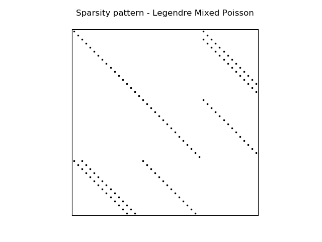
Note that each item in (13) is a collection of instances of the TPMatrix class, and for similar reasons as given around (4), we get also here one regular block matrix for each Fourier wavenumber. The sparsity pattern is the same for all matrices except for wavenumber 0. The (highly sparse) sparsity pattern for block matrix \(H\) with wavenumber \(\ne 0\) is shown in the image below

A complete demo for the coupled problem discussed here can be found in MixedPoisson.py and a 3D version is in MixedPoisson3D.py.

Integrators

The integrators module contains some interator classes that can be used to integrate a solution forward in time. Integrators are set up to solve initial value problems like

(14)\[\frac{\partial u}{\partial t} = L u + N(u)\]

where \(u\) is the solution, \(L\) is a linear operator and \(N(u)\) is the nonlinear part of the right hand side.

There are two kinds of integrators, or time steppers. The first are ment to be subclassed and used one at the time. These are

• IRK3: Third order implicit Runge-Kutta

• RK4: Explicit Runge-Kutta fourth order (Fourier only)

• ETD: Exponential time differencing Euler method (Fourier only)

• ETDRK4: Exponential time differencing Runge-Kutta fourth order (Fourier only)

See, e.g.:

H. Montanelli and N. Bootland "Solving periodic semilinear PDEs in 1D, 2D and
3D with exponential integrators", https://arxiv.org/pdf/1604.08900.pdf

The second kind is ment to be used for systems of equations, one class instance for each equation. These are mainly IMEX Runge Kutta integrators:

• IMEXRK3

• IMEXRK111

• IMEXRK222

• IMEXRK443

See, e.g., https://github.com/spectralDNS/shenfun/blob/master/demo/ChannelFlow.py for an example of use for the Navier-Stokes equations. The IMEX solvers are described by:

Ascher, Ruuth and Spiteri 'Implicit-explicit Runge-Kutta methods for
time-dependent partial differential equations' Applied Numerical
Mathematics, 25 (1997) 151-167

Note that the IMEX solvers are intended for use with problems consisting of one non-periodic direction.

To illustrate, we consider the time-dependent 1-dimensional Kortveeg-de Vries equation

\[\frac{\partial u}{\partial t} + \frac{\partial ^3 u}{\partial x^3} + u \frac{\partial u}{\partial x} = 0\]

which can also be written as

\[\frac{\partial u}{\partial t} + \frac{\partial ^3 u}{\partial x^3} + \frac{1}{2}\frac{\partial u^2}{\partial x} = 0\]

We neglect boundary issues and choose a periodic domain \([0, 2\pi)\) with Fourier exponentials as test functions. The initial condition is chosen as

(15)\[ u(x, t=0) = 3 A^2/\cosh(0.5 A (x-\pi+2))^2 + 3B^2/\cosh(0.5B(x-\pi+1))^2\]

where \(A\) and \(B\) are constants. For discretization in space we use the basis \(V_N = \text{span}\{exp(\imath k x)\}_{k=0}^N\) and formulate the variational problem: find \(u \in V_N\) such that

\[\frac{\partial }{\partial t} \Big(u, v \Big) = -\Big(\frac{\partial^3 u }{\partial x^3}, v \Big) - \Big(\frac{1}{2}\frac{\partial u^2}{\partial x}, v\Big), \quad \forall v \in V_N\]

We see that the first term on the right hand side is linear in \(u\), whereas the second term is nonlinear. To implement this problem in shenfun we start by creating the necessary basis and test and trial functions

import numpy as np
from shenfun import *

N = 256
T = FunctionSpace(N, 'F', dtype='d')
u = TrialFunction(T)
v = TestFunction(T)
u_ = Array(T)
u_hat = Function(T)

We then create two functions representing the linear and nonlinear part of (14):

def LinearRHS(self, u, **params):
    return -Dx(u, 0, 3)

k = T.wavenumbers(scaled=True, eliminate_highest_freq=True)
def NonlinearRHS(self, u, u_hat, rhs, **params):
    rhs.fill(0)
    u_[:] = T.backward(u_hat, u_)
    rhs = T.forward(-0.5*u_**2, rhs)
    rhs *= 1j*k
    return rhs   # return inner(grad(-0.5*Up**2), v)

Note that we differentiate in NonlinearRHS by using the wavenumbers k directly. Alternative notation, that is given in commented out text, is slightly slower, but the results are the same.

The solution vector u_ needs also to be initialized according to (15)

A = 25.
B = 16.
x = T.points_and_weights()[0]
u_[:] = 3*A**2/np.cosh(0.5*A*(x-np.pi+2))**2 + 3*B**2/np.cosh(0.5*B*(x-np.pi+1))**2
u_hat = T.forward(u_, u_hat)

Finally we create an instance of the ETDRK4 solver, and integrate forward with a given timestep

dt = 0.01/N**2
end_time = 0.006
integrator = ETDRK4(T, L=LinearRHS, N=NonlinearRHS)
integrator.setup(dt)
u_hat = integrator.solve(u_, u_hat, dt, (0, end_time))

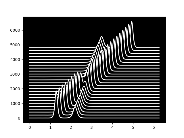
The solution is two waves travelling through eachother, seemingly undisturbed. See kdv.py for more details.

MPI

Shenfun makes use of the Message Passing Interface (MPI) to solve problems on distributed memory architectures. OpenMP is also possible to enable for FFTs.

Dataarrays in Shenfun are distributed using a new and completely generic method, that allows for any index of a multidimensional array to be distributed. To illustrate, lets consider a TensorProductSpace of three dimensions, such that the arrays living in this space will be 3-dimensional. We create two spaces that are identical, except from the MPI decomposition, and we use 4 CPUs (mpirun -np 4 python mpitest.py, if we store the code in this section as mpitest.py):

from shenfun import *
from mpi4py_fft import generate_xdmf
N = (20, 40, 60)
K0 = FunctionSpace(N[0], 'F', dtype='D', domain=(0, 1))
K1 = FunctionSpace(N[1], 'F', dtype='D', domain=(0, 2))
K2 = FunctionSpace(N[2], 'F', dtype='d', domain=(0, 3))
T0 = TensorProductSpace(comm, (K0, K1, K2), axes=(0, 1, 2), slab=True)
T1 = TensorProductSpace(comm, (K0, K1, K2), axes=(1, 0, 2), slab=True)

Here the keyword slab determines that only one index set of the 3-dimensional arrays living in T0 or T1 should be distributed. The defaul is to use two, which corresponds to a so-called pencil decomposition. The axes-keyword determines the order of which transforms are conducted, starting from last to first in the given tuple. Note that T0 now will give arrays in real physical space that are distributed in the first index, whereas T1 will give arrays that are distributed in the second. This is because 0 and 1 are the first items in the tuples given to axes.

We can now create some Arrays on these spaces:

u0 = Array(T0, val=comm.Get_rank())
u1 = Array(T1, val=comm.Get_rank())

such that u0 and u1 have values corresponding to their communicating processors rank in the COMM_WORLD group (the group of all CPUs).

Note that both the TensorProductSpaces have functions with expansion

(16)\[ u(x, y, z) = \sum_{l=-N_0/2}^{N_0/2-1}\sum_{m=-N_1/2}^{N_1/2-1}\sum_{n=0}^{N_2/2} \hat{u}_{l,m,n} e^{\imath (lx + my + nz)}.\]

where \(u(x, y, z)\) is the continuous solution in real physical space, and \(\hat{u}\) are the spectral expansion coefficients. Note that the last axis has index set different from the two others because the input data is real. If we evaluate expansion (16) on the real physical mesh, then we get

(17)\[ u(x_i, y_j, z_k) = \sum_{l=-N_0/2}^{N_0/2-1}\sum_{m=-N_1/2}^{N_1/2-1}\sum_{n=0}^{N_2/2} \hat{u}_{l,m,n} e^{\imath (lx_i + my_j + nz_k)}.\]

The function \(u(x_i, y_j, z_k)\) corresponds to the arrays u0, u1, whereas we have not yet computed the array \(\hat{u}\). We could get \(\hat{u}\) as:

u0_hat = Function(T0)
u0_hat = T0.forward(u0, u0_hat)

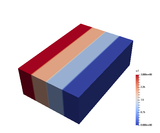
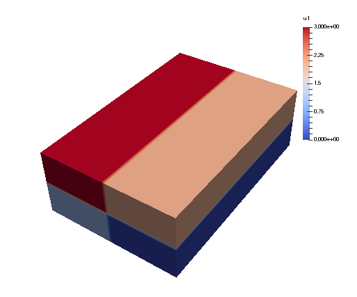
Now, u0 and u1 have been created on the same mesh, which is a structured mesh of shape \((20, 40, 60)\). However, since they have different MPI decomposition, the values used to fill them on creation will differ. We can visualize the arrays in Paraview using some postprocessing tools, to be further described in Sec Postprocessing:

u0.write('myfile.h5', 'u0', 0, domain=T0.mesh())
u1.write('myfile.h5', 'u1', 0, domain=T1.mesh())
if comm.Get_rank() == 0:
    generate_xdmf('myfile.h5')

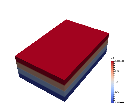
And when the generated myfile.xdmf is opened in Paraview, we can see the different distributions. The function u0 is shown first, and we see that it has different values along the short first dimension. The second figure is evidently distributed along the second dimension. Both arrays are non-distributed in the third and final dimension, which is fortunate, because this axis will be the first to be transformed in, e.g., u0_hat = T0.forward(u0, u0_hat).

We can now decide to distribute not just one, but the first two axes using a pencil decomposition instead. This is achieved simply by dropping the slab keyword:

T2 = TensorProductSpace(comm, (K0, K1, K2), axes=(0, 1, 2))
u2 = Array(T2, val=comm.Get_rank())
u2.write('pencilfile.h5', 'u2', 0)
if comm.Get_rank() == 0:
    generate_xdmf('pencilfile.h5')

Running again with 4 CPUs the array u2 will look like:

The local slices into the global array may be obtained through:

>>> print(comm.Get_rank(), T2.local_slice(False))
0 [slice(0, 10, None), slice(0, 20, None), slice(0, 60, None)]
1 [slice(0, 10, None), slice(20, 40, None), slice(0, 60, None)]
2 [slice(10, 20, None), slice(0, 20, None), slice(0, 60, None)]
3 [slice(10, 20, None), slice(20, 40, None), slice(0, 60, None)]

In spectral space the distribution will be different. This is because the discrete Fourier transforms are performed one axis at the time, and for this to happen the dataarrays need to be realigned to get entire axis available for each processor. Naturally, for the array in the pencil example (see image), we can only perform an FFT over the third and longest axis, because only this axis is locally available to all processors. To do the other directions, the dataarray must be realigned and this is done internally by the TensorProductSpace class. The shape of the datastructure in spectral space, that is the shape of \(\hat{u}\), can be obtained as:

>>> print(comm.Get_rank(), T2.local_slice(True))
0 [slice(0, 20, None), slice(0, 20, None), slice(0, 16, None)]
1 [slice(0, 20, None), slice(0, 20, None), slice(16, 31, None)]
2 [slice(0, 20, None), slice(20, 40, None), slice(0, 16, None)]
3 [slice(0, 20, None), slice(20, 40, None), slice(16, 31, None)]

Evidently, the spectral space is distributed in the last two axes, whereas the first axis is locally avalable to all processors. Tha dataarray is said to be aligned in the first dimension.

Post processing

MPI is great because it means that you can run Shenfun on pretty much as many CPUs as you can get your hands on. However, MPI makes it more challenging to do visualization, in particular with Python and Matplotlib. For this reason there is a utilities module with helper classes for dumping dataarrays to HDF5 or NetCDF

Most of the IO has already been implemented in mpi4py-fft. The classes HDF5File and NCFile are used exactly as they are implemented in mpi4py-fft. As a common interface we provide

• ShenfunFile()

where ShenfunFile() returns an instance of either HDF5File or NCFile, depending on choice of backend.

For example, to create an HDF5 writer for a 3D TensorProductSpace with Fourier bases in all directions:

from shenfun import *
from mpi4py import MPI
N = (24, 25, 26)
K0 = FunctionSpace(N[0], 'F', dtype='D')
K1 = FunctionSpace(N[1], 'F', dtype='D')
K2 = FunctionSpace(N[2], 'F', dtype='d')
T = TensorProductSpace(MPI.COMM_WORLD, (K0, K1, K2))
fl = ShenfunFile('myh5file', T, backend='hdf5', mode='w')

The file instance fl will now have two method that can be used to either write dataarrays to file, or read them back again.

• fl.write

• fl.read

With the HDF5 backend we can write both arrays from physical space (Array), as well as spectral space (Function). However, the NetCDF4 backend cannot handle complex dataarrays, and as such it can only be used for real physical dataarrays.

In addition to storing complete dataarrays, we can also store any slices of the arrays. To illustrate, this is how to store three snapshots of the u array, along with some global 2D and 1D slices:

u = Array(T)
u[:] = np.random.random(u.shape)
d = {'u': [u, (u, np.s_[4, :, :]), (u, np.s_[4, 4, :])]}
fl.write(0, d)
u[:] = 2
fl.write(1, d)

The ShenfunFile may also be used for the CompositeSpace, or VectorSpace, that are collections of the scalar TensorProductSpace. We can create a CompositeSpace consisting of two TensorProductSpaces, and an accompanying writer class as:

TT = CompositeSpace([T, T])
fl_m = ShenfunFile('mixed', TT, backend='hdf5', mode='w')

Let’s now consider a transient problem where we step a solution forward in time. We create a solution array from the Array class, and update the array inside a while loop:

TT = VectorSpace(T)
fl_m = ShenfunFile('mixed', TT, backend='hdf5', mode='w')
u = Array(TT)
tstep = 0
du = {'uv': (u,
            (u, [4, slice(None), slice(None)]),
            (u, [slice(None), 10, 10]))}
while tstep < 3:
    fl_m.write(tstep, du, forward_output=False)
    tstep += 1

Note that on each time step the arrays u, (u, [4, slice(None), slice(None)]) and (u, [slice(None), 10, 10]) are vectors, and as such of global shape (3, 24, 25, 26), (3, 25, 26) and (3, 25), respectively. However, they are stored in the hdf5 file under their spatial dimensions 1D, 2D and 3D, respectively.

Note that the slices in the above dictionaries are global views of the global arrays, that may or may not be distributed over any number of processors. Also note that these routines work with any number of CPUs, and the number of CPUs does not need to be the same when storing or retrieving the data.

After running the above, the different arrays will be found in groups stored in myh5file.h5 with directory tree structure as:

myh5file.h5/
└─ u/
   ├─ 1D/
   |  └─ 4_4_slice/
   |     ├─ 0
   |     └─ 1
   ├─ 2D/
   |  └─ 4_slice_slice/
   |     ├─ 0
   |     └─ 1
   ├─ 3D/
   |  ├─ 0
   |  └─ 1
   └─ mesh/
      ├─ x0
      ├─ x1
      └─ x2

Likewise, the mixed.h5 file will at the end of the loop look like:

mixed.h5/
└─ uv/
   ├─ 1D/
   |  └─ slice_10_10/
   |     ├─ 0
   |     ├─ 1
   |     └─ 3
   ├─ 2D/
   |  └─ 4_slice_slice/
   |     ├─ 0
   |     ├─ 1
   |     └─ 3
   ├─ 3D/
   |  ├─ 0
   |  ├─ 1
   |  └─ 3
   └─ mesh/
      ├─ x0
      ├─ x1
      └─ x2

Note that the mesh is stored as well as the results. The three mesh arrays are all 1D arrays, representing the domain for each basis in the TensorProductSpace.

With NetCDF4 the layout is somewhat different. For mixed above, if we were using backend netcdf instead of hdf5, we would get a datafile where ncdump -h mixed.nc would result in:

netcdf mixed {
dimensions:
        time = UNLIMITED ; // (3 currently)
        i = 3 ;
        x = 24 ;
        y = 25 ;
        z = 26 ;
variables:
        double time(time) ;
        double i(i) ;
        double x(x) ;
        double y(y) ;
        double z(z) ;
        double uv(time, i, x, y, z) ;
        double uv_4_slice_slice(time, i, y, z) ;
        double uv_slice_10_10(time, i, x) ;
}

Note that it is also possible to store vector arrays as scalars. For NetCDF4 this is necessary for direct visualization using Visit. To store vectors as scalars, simply use:

fl_m.write(tstep, du, forward_output=False, as_scalar=True)

ParaView

The stored datafiles can be visualized in ParaView. However, ParaView cannot understand the content of these HDF5-files without a little bit of help. We have to explain that these data-files contain structured arrays of such and such shape. The way to do this is through the simple XML descriptor XDMF. To this end there is a function imported from mpi4py-fft called generate_xdmf that can be called with any one of the generated hdf5-files:

generate_xdmf('myh5file.h5')
generate_xdmf('mixed.h5')

This results in some light xdmf-files being generated for the 2D and 3D arrays in the hdf5-file:

• myh5file.xdmf

• myh5file_4_slice_slice.xdmf

• mixed.xdmf

• mixed_4_slice_slice.xdmf

These xdmf-files can be opened and inspected by ParaView. Note that 1D arrays are not wrapped, and neither are 4D.

An annoying feature of Paraview is that it views a three-dimensional array of shape \((N_0, N_1, N_2)\) as transposed compared to shenfun. That is, for Paraview the last axis represents the \(x\)-axis, whereas shenfun (like most others) considers the first axis to be the \(x\)-axis. So when opening a three-dimensional array in Paraview one needs to be aware. Especially when plotting vectors. Assume that we are working with a Navier-Stokes solver and have a three-dimensional VectorSpace to represent the fluid velocity:

from mpi4py import MPI
from shenfun import *

comm = MPI.COMM_WORLD
N = (32, 64, 128)
V0 = FunctionSpace(N[0], 'F', dtype='D')
V1 = FunctionSpace(N[1], 'F', dtype='D')
V2 = FunctionSpace(N[2], 'F', dtype='d')
T = TensorProductSpace(comm, (V0, V1, V2))
TV = VectorSpace(T)
U = Array(TV)
U[0] = 0
U[1] = 1
U[2] = 2

To store the resulting Array U we can create an instance of the HDF5File class, and store using keyword as_scalar=True:

hdf5file = ShenfunFile("NS", TV, backend='hdf5', mode='w')
...
file.write(0, {'u': [U]}, as_scalar=True)
file.write(1, {'u': [U]}, as_scalar=True)

Alternatively, one may store the arrays directly as:

U.write('U.h5', 'u', 0, domain=T.mesh(), as_scalar=True)
U.write('U.h5', 'u', 1, domain=T.mesh(), as_scalar=True)

Generate an xdmf file through:

generate_xdmf('NS.h5')

and open the generated NS.xdmf file in Paraview. You will then see three scalar arrays u0, u1, u2, each one of shape (32, 64, 128), for the vector component in what Paraview considers the \(z\), \(y\) and \(x\) directions, respectively. Other than the swapped coordinate axes there is no difference. But be careful if creating vectors in Paraview with the Calculator. The vector should be created as:

u0*kHat+u1*jHat+u2*iHat