Demo - Cubic nonlinear Klein-Gordon equation

Authors:

Mikael Mortensen (mikaem at math.uio.no)

Date:

April 13, 2018

Summary. This is a demonstration of how the Python module shenfun can be used to solve the time-dependent, nonlinear Klein-Gordon equation, in a triply periodic domain. The demo is implemented in a single Python file KleinGordon.py, and it may be run in parallel using MPI. The Klein-Gordon equation is solved using a mixed formulation. The discretization, and some background on the spectral Galerkin method is given first, before we turn to the actual details of the shenfun implementation.

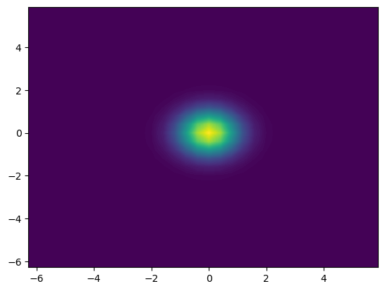
Movie showing the evolution of the solution \(u\) from Eq. (1), in a slice through the center of the domain, computed with the code described in this demo.

The nonlinear Klein-Gordon equation

The cubic nonlinear Klein-Gordon equation is a wave equation important for many scientific applications such as solid state physics, nonlinear optics and quantum field theory [Waz08]. The equation is given as

(1)\[ \frac{\partial^2 u}{\partial t^2} = \nabla^2 u - \gamma(u - u|u|^2) \quad \text{for} \, u \in \Omega,\]

with initial conditions

(2)\[ u(\boldsymbol{x}, t=0) = u^0 \quad \text{and} \quad \frac{\partial u(\boldsymbol{x}, t=0)}{\partial t} = u_t^0.\]

The spatial coordinates are here denoted as \(\boldsymbol{x} = (x, y, z)\), and \(t\) is time. The parameter \(\gamma=\pm 1\) determines whether the equations are focusing (\(+1\)) or defocusing (\(-1\)) (in the movie we have used \(\gamma=1\)). The domain \(\Omega=[-2\pi, 2\pi)^3\) is triply periodic and initial conditions will here be set as

(3)\[ u^0 = 0.1 \exp \left( -\boldsymbol{x} \cdot \boldsymbol{x} \right),\]

(4)\[ u_t^0 = 0.\]

We will solve these equations using a mixed formulation and a spectral Galerkin method. The mixed formulation reads

(5)\[ \frac{\partial f}{\partial t} = \nabla^2 u - \gamma (u - u|u|^2),\]

(6)\[ \frac{\partial u}{\partial t} = f.\]

The energy of the solution can be computed as

(7)\[ E(u) = \int_{\Omega} \left( \frac{1}{2} f^2 + \frac{1}{2}|\nabla u|^2 + \gamma(\frac{1}{2}u^2 - \frac{1}{4}u^4) \right) dx\]

and it is crucial that this energy remains constant in time.

The movie above is showing the solution \(u\), computed with the code shown below.

Spectral Galerkin formulation

The PDEs in (5) and (6) can be solved with many different numerical methods. We will here use the shenfun software and this software makes use of the spectral Galerkin method. Being a Galerkin method, we need to reshape the governing equations into proper variational forms, and this is done by multiplying (5) and (6) with the complex conjugate of proper test functions and then integrating over the domain. To this end we make use of the triply periodic tensor product function space \(W^{\boldsymbol{N}}(\Omega)\) (defined in Eq. (14)) and use testfunctions \(g \in W^{\boldsymbol{N}}\) with Eq. (5) and \(v \in W^{\boldsymbol{N}}\) with Eq. (6), and obtain

(8)\[ \frac{\partial}{\partial t} \int_{\Omega} f\, \overline{g}\, w \,d\Omega = \int_{\Omega} \left(\nabla^2 u - \gamma( u\, - u|u|^2) \right) \overline{g} \, w \,d\Omega,\]

(9)\[ \frac{\partial }{\partial t} \int_{\Omega} u\, \overline{v}\, w \, dx = \int_{\Omega} f\, \overline{v} \, w \, d\Omega.\]

Note that the overline is used to indicate a complex conjugate, and \(w\) is a weight function associated with the test functions. The functions \(f\) and \(u\) are now to be considered as trial functions, and the integrals over the domain are referred to as inner products. With inner product notation

\[\left(u, v\right) = \int_{\Omega} u \, \overline{v} \, w\, dx.\]

and an integration by parts on the Laplacian, the variational problem can be formulated as:

(10)\[ \frac{\partial}{\partial t} (f, g) = -(\nabla u, \nabla g) -\gamma \left( u - u|u|^2, g \right),\]

(11)\[ \frac{\partial }{\partial t} (u, v) = (f, v).\]

The time and space discretizations are still left open. There are numerous different approaches that one could take for discretizing in time, and the first two terms on the right hand side of (10) can easily be treated implicitly as well as explicitly. However, the approach we will follow in Sec. (Runge-Kutta integrator) is a fully explicit 4th order Runge-Kutta method. Also note that the inner product in the demo will be computed numerically with quadrature through fast Fourier transforms, and the integrals are thus not computed exactly for all terms.

Discretization

To find a numerical solution we need to discretize the continuous problem (10) and (11) in space as well as time. Since the problem is triply periodic, Fourier exponentials are normally the best choice for trial and test functions, and as such we use basis functions

(12)\[ \phi_l(x) = e^{\imath \underline{l} x}, \quad -\infty < l < \infty,\]

where \(l\) is the wavenumber, and \(\underline{l}=\frac{2\pi}{L}l\) is the scaled wavenumber, scaled with domain length \(L\) (here \(4\pi\)). Since we want to solve these equations on a computer, we need to choose a finite number of test functions. A function space \(V^N\) can be defined as

(13)\[ V^N(x) = \text{span} \{\phi_l(x)\}_{l\in \boldsymbol{l}},\]

where \(N\) is chosen as an even positive integer and \(\boldsymbol{l} = -N/2, -N/2+1, \ldots, N/2-1\). And now, since \(\Omega\) is a three-dimensional domain, we can create tensor products of such bases to get, e.g., for three dimensions

(14)\[ W^{\boldsymbol{N}}(x, y, z) = V^N(x) \otimes V^N(y) \otimes V^N(z),\]

where \(\boldsymbol{N} = (N, N, N)\). Obviously, it is not necessary to use the same number (\(N\)) of basis functions for each direction, but it is done here for simplicity. A 3D tensor product basis function is now defined as

(15)\[ \Phi_{lmn}(x,y,z) = e^{\imath \underline{l} x} e^{\imath \underline{m} y} e^{\imath \underline{n} z} = e^{\imath (\underline{l}x + \underline{m}y + \underline{n}z)},\]

where the indices for \(y\)- and \(z\)-direction are \(\underline{m}=\frac{2\pi}{L}m, \underline{n}=\frac{2\pi}{L}n\), and \(\boldsymbol{m}\) and \(\boldsymbol{n}\) are the same as \(\boldsymbol{l}\) due to using the same number of basis functions for each direction. One distinction, though, is that for the \(z\)-direction expansion coefficients are only stored for \(n=0, 1, \ldots, N/2\) due to Hermitian symmetry (real input data). However, for simplicity, we still write the sum in Eq. (16) over the entire range of basis functions.

We now look for solutions of the form

(16)\[ u(x, y, z, t) = \sum_{l=-N/2}^{N/2-1}\sum_{m=-N/2}^{N/2-1}\sum_{n=-N/2}^{N/2-1} \hat{u}_{lmn} (t)\Phi_{lmn}(x,y,z).\]

The expansion coefficients \(\hat{\boldsymbol{u}} = \{\hat{u}_{lmn}(t)\}_{(l,m,n) \in \boldsymbol{l} \times \boldsymbol{m} \times \boldsymbol{n}}\) can be related directly to the solution \(u(x, y, z, t)\) using Fast Fourier Transforms (FFTs) if we are satisfied with obtaining the solution in quadrature points corresponding to

(17)\[ x_i = \frac{4 \pi i}{N}-2\pi \quad \forall \, i \in \boldsymbol{i}, \text{where}\, \boldsymbol{i}=(0,1,\ldots,N-1),\]

(18)\[ y_j = \frac{4 \pi j}{N}-2\pi \quad \forall \, j \in \boldsymbol{j}, \text{where}\, \boldsymbol{j}=(0,1,\ldots,N-1),\]

(19)\[ z_k = \frac{4 \pi k}{N}-2\pi \quad \forall \, k \in \boldsymbol{k}, \text{where}\, \boldsymbol{k}=(0,1,\ldots,N-1).\]

Note that these points are different from the standard (like \(2\pi j/N\)) since the domain is set to \([-2\pi, 2\pi]^3\) and not the more common \([0, 2\pi]^3\). We have

(20)\[ \boldsymbol{u} = \mathcal{F}_x^{-1}\left(\mathcal{F}_y^{-1}\left(\mathcal{F}_z^{-1}\left(\hat{\boldsymbol{u}}\right)\right)\right)\]

with \(\boldsymbol{u} = \{u(x_i, y_j, z_k)\}_{(i,j,k)\in \boldsymbol{i} \times \boldsymbol{j} \times \boldsymbol{k}}\) and where \(\mathcal{F}_x^{-1}\) is the inverse Fourier transform along the direction \(x\), for all indices in the other direction. Note that the three inverse FFTs are performed sequentially, one direction at the time, and that there is no scaling factor due to the definition used for the inverse Fourier transform

(21)\[ u(x_j) = \sum_{l=-N/2}^{N/2-1} \hat{u}_l e^{\imath \underline{l} x_j}, \quad \,\, \forall \, j \in \, \boldsymbol{j}.\]

Note that this differs from the definition used by, e.g., Numpy.

The inner products used in Eqs. (10), (11) may be computed using forward FFTs. However, there is a tiny detail that deserves a comment. The regular Fourier inner product is given as

\[\int_{0}^{L} e^{\imath \underline{k}x} e^{- \imath \underline{l}x} dx = L\, \delta_{kl}\]

where a weight function is chosen as \(w(x) = 1\) and \(\delta_{kl}\) equals unity for \(k=l\) and zero otherwise. In Shenfun we choose instead to use a weight function \(w(x)=1/L\), such that the weighted inner product integrates to unity:

\[\int_{0}^{L} e^{\imath \underline{k}x} e^{- \imath \underline{l}x} \frac{1}{L} dx = \delta_{kl}.\]

With this weight function the (discrete) scalar product and the forward transform are the same and we obtain:

(22)\[ \left(u, v \right) = \boldsymbol{\hat{u}} = \left(\frac{1}{N}\right)^3 \mathcal{F}_z\left(\mathcal{F}_y\left(\mathcal{F}_x\left(\boldsymbol{u}\right)\right)\right).\]

From this we see that the variational forms (10) and (11) may be written in terms of the Fourier transformed quantities \(\hat{\boldsymbol{u}}\) and \(\hat{\boldsymbol{f}}\). Expanding the exact derivatives of the nabla operator, we have

(23)\[ (\nabla u, \nabla v) = \left((\underline{l}^2+\underline{m}^2+\underline{n}^2)\hat{u}_{lmn}\right),\]

(24)\[ (u, v) = \left(\hat{u}_{lmn}\right),\]

(25)\[ (u|u|^2, v) = \left(\widehat{u|u|^2}_{lmn}\right)\]

where the indices on the right hand side run over \((l, m, n) \in \boldsymbol{l} \times \boldsymbol{m} \times \boldsymbol{n}\). The equations to be solved for each wavenumber can now be found directly as

(26)\[ \frac{\partial \hat{f}_{lmn}}{\partial t} = \left(-(\underline{l}^2+\underline{m}^2+\underline{n}^2+\gamma)\hat{u}_{lnm} + \gamma \widehat{u|u|^2}_{lnm}\right),\]

(27)\[ \frac{\partial \hat{u}_{lnm}}{\partial t} = \hat{f}_{lnm}.\]

There is more than one way to arrive at these equations. Taking the 3D Fourier transform of both equations (5) and (6) is one obvious way. With the Python module shenfun, one can work with the inner products as seen in (10) and (11), or the Fourier transforms directly. See for example Sec. Runge-Kutta integrator for how \((\nabla u, \nabla v)\) can be implemented. In short, shenfun contains all the tools required to work with the spectral Galerkin method, and we will now see how shenfun can be used to solve the Klein-Gordon equation.

For completion, we note that the discretized problem to solve can be formulated with the Galerkin method as: for all \(t>0\), find \((f, u) \in W^N \times W^N\) such that

(28)\[ \frac{\partial}{\partial t} (f, g) = -(\nabla u, \nabla g) -\gamma \left( u - u|u|^2, g \right) \quad \forall \, g \in W^{N},\]

(29)\[ \frac{\partial }{\partial t} (u, v) = (f, v) \quad \forall \, v \in W^N.\]

where \(u(x, y, z, 0)\) and \(f(x, y, z, 0)\) are given as the initial conditions according to Eq. (2).

Implementation

To solve the Klein-Gordon equations we need to make use of the Fourier function spaces defined in shenfun, and these are found in submodule shenfun.fourier.bases. The triply periodic domain allows for Fourier in all three directions, and we can as such create one instance of this space using FunctionSpace() with family Fourier for each direction. However, since the initial data are real, we can take advantage of Hermitian symmetries and thus make use of a real to complex class for one (but only one) of the directions, by specifying dtype='d'. We can only make use of the real-to-complex class for the direction that we choose to transform first with the forward FFT, and the reason is obviously that the output from a forward transform of real data is now complex. We may start implementing the solver as follows

from shenfun import *
import numpy as np
import sympy as sp

# Set size of discretization
N = (32, 32, 32)

# Defocusing or focusing
gamma = 1

rank = comm.Get_rank()

# Create function spaces
K0 = FunctionSpace(N[0], 'F', domain=(-2*np.pi, 2*np.pi), dtype='D')
K1 = FunctionSpace(N[1], 'F', domain=(-2*np.pi, 2*np.pi), dtype='D')
K2 = FunctionSpace(N[2], 'F', domain=(-2*np.pi, 2*np.pi), dtype='d')

We now have three instances K0, K1 and K2, corresponding to the space (13), that each can be used to solve one-dimensional problems. However, we want to solve a 3D problem, and for this we need a tensor product space, like (14), created as a tensor product of these three spaces

T = TensorProductSpace(comm, (K0, K1, K2), **{'planner_effort':
                                              'FFTW_MEASURE'})

Here the planner_effort, which is a flag used by FFTW, is optional. Possibel choices are from the list (FFTW_ESTIMATE, FFTW_MEASURE, FFTW_PATIENT, FFTW_EXHAUSTIVE), and the flag determines how much effort FFTW puts in looking for an optimal algorithm for the current platform. Note that it is also possible to use FFTW wisdom with shenfun, and as such, for production, one may perform exhaustive planning once and then simply import the result of that planning later, as wisdom.

The TensorProductSpace instance T contains pretty much all we need for computing inner products or fast transforms between real and wavenumber space. However, since we are going to solve for a mixed system, it is convenient to also use the CompositeSpace class

TT = CompositeSpace([T, T])
TV = VectorSpace(T)

Here the space TV will be used to compute gradients, which explains why it is a vector.

We need containers for the solution as well as intermediate work arrays for, e.g., the Runge-Kutta method. Arrays are created using Sympy for initialization. Below f is initialized to 0, whereas u = 0.1*sp.exp(-(x**2 + y**2 + z**2)).

# Use sympy to set up initial condition
x, y, z = sp.symbols("x,y,z", real=True)
ue = 0.1*sp.exp(-(x**2 + y**2 + z**2))

fu = Array(TT, buffer=(0, ue)) # Solution array in physical space
f, u = fu                # Split solution array by creating two views u and f
dfu = Function(TT)       # Array for right hand sides
df, du = dfu             # Split into views
Tp = T.get_dealiased((1.5, 1.5, 1.5))
up = Array(Tp)           # Work array

fu_hat = Function(TT)    # Solution in spectral space
fu_hat = fu.forward()
f_hat, u_hat = fu_hat

gradu = Array(TV)        # Solution array for gradient

The Array class is a subclass of Numpy’s ndarray, without much more functionality than constructors that return arrays of the correct shape according to the basis used in the construction. The Array represents the left hand side of (16), evaluated on the quadrature mesh. A different type of array is returned by the Function class, that subclasses both Nympy’s ndarray as well as an internal BasisFunction class. An instance of the Function represents the entire spectral Galerkin function (16).

Runge-Kutta integrator

We use an explicit fourth order Runge-Kutta integrator, imported from shenfun.utilities.integrators. The solver requires one function to compute nonlinear terms, and one to compute linear. But here we will make just one function that computes both, and call it NonlinearRHS:

uh = TrialFunction(T)
vh = TestFunction(T)
L = inner(grad(vh), -grad(uh)) + [inner(vh, -gamma*uh)]
L = la.SolverDiagonal(L).mat.scale

def NonlinearRHS(self, fu, fu_hat, dfu_hat, **par):
    global count, up
    dfu_hat.fill(0)
    f_hat, u_hat = fu_hat
    df_hat, du_hat = dfu_hat
    up = Tp.backward(u_hat, up)
    df_hat = Tp.forward(gamma*up**3, df_hat)
    df_hat += L*u_hat
    du_hat[:] = f_hat
    return dfu_hat

Note that L now is an array that represents the linear coefficients in (27).

All that is left is to write a function that is called on each time step, which will allow us to store intermediate solutions, compute intermediate energies, and plot intermediate solutions. Since we will plot the same plot many times, we create the figure first, and then simply update the plotted arrays in the update function.

import matplotlib.pyplot as plt
X = T.local_mesh(True)
if rank == 0:
    plt.figure()
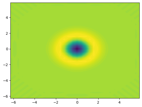
    image = plt.contourf(X[1][..., 0], X[0][..., 0], u[..., N[2]//2], 100)
    plt.draw()
    plt.pause(1e-6)

The actual update function is

# Get wavenumbers
K = np.array(T.local_wavenumbers(True, True, True))

def update(self, fu, fu_hat, t, tstep, **params):
    global gradu

    transformed = False
    if rank == 0 and tstep % params['plot_tstep'] == 0 and params['plot_tstep'] > 0:
        fu = fu_hat.backward(fu)
        f, u = fu[:]
        image.axes.clear()
        image.axes.contourf(X[1][..., 0], X[0][..., 0], u[..., N[2]//2], 100)
        plt.pause(1e-6)
        transformed = True

    if tstep % params['Compute_energy'] == 0:
        if transformed is False:
            fu = fu_hat.backward(fu)
        f, u = fu
        f_hat, u_hat = fu_hat
        ekin = 0.5*energy_fourier(f_hat, T)
        es = 0.5*energy_fourier(1j*(K*u_hat), T)
        eg = gamma*np.sum(0.5*u**2 - 0.25*u**4)/np.prod(np.array(N))
        eg = comm.allreduce(eg)
        gradu = TV.backward(1j*(K[0]*u_hat[0]+K[1]*u_hat[1]+K[2]*u_hat[2]), gradu)
        ep = comm.allreduce(np.sum(f*gradu)/np.prod(np.array(N)))
        ea = comm.allreduce(np.sum(np.array(X)*(0.5*f**2 + 0.5*gradu**2 - (0.5*u**2 - 0.25*u**4)*f))/np.prod(np.array(N)))
        if rank == 0:
            print("Time = %2.2f Total energy = %2.8e Linear momentum %2.8e Angular momentum %2.8e" %(t, ekin+es+eg, ep, ea))
        comm.barrier()

With all functions in place, the actual integrator can be created and called as

par = {'Compute_energy': 10,
       'plot_tstep': 10,
       'end_time': 1}
dt = 0.005
integrator = RK4(TT, N=NonlinearRHS, update=update, **par)
integrator.setup(dt)
fu_hat = integrator.solve(fu, fu_hat, dt, (0, par['end_time']))

A complete solver is found here.